Daily Digest — 2026-06-11
26 newsletters today.
In this digest
- Abandoned Futures — The Yakovlev Yak-38 Forger and the Yak-41 Freestyle: The Soviet Supersonic VTOL Fighter That Beat the F-35B by 30 Years and Got Killed by the Collapse of the USSR
- ArXiv Paper Digest — Understanding and Detecting Scalability Faults in Large-Scale Distributed Systems
- Daily Automotive Engines — Turbocharger Compressor Wheel Hub-to-Tip Ratio: Why Inducer Geometry Limits Flow
- Daily Debugging Puzzle — Rust's Vec::retain Index Trap: The Predicate That Forgets Where It Is
- Daily Digital Circuits — Skewed CMOS and High-Speed Domino Output Drivers
- Daily Electrical Circuits — Hot-Swap Controllers: Safely Inserting Boards into Live Backplanes
- Daily Engineering Lesson — Metal Injection Molding (MIM): Powder Metallurgy Meets Plastic Injection Molding for Small, Complex Steel Parts
- Forgotten Books — The 1827 Veterinarian Who Demanded Evidence Over Recipes
- Forgotten Darkroom — The Photographer's Paradox: Why Mastering One Process Beat Trying Them All
- Forgotten Patent — Oliver Heaviside's "Loaded Line" Patent: The 1887 Invention That Made Long-Distance Telephony Possible — and Quietly Shaped Every DSL Modem
- Daily GitHub Zero Stars — jmandel/voxtral-dictate
- Daily Hardware Architecture — The Reorder Buffer's Width vs. Depth Tradeoff: Why CPUs Can't Just Get Bigger
- Hacker News Deep Cuts — Model choice is not an authorization layer
- HN Jobs Teardown — joyn.de: What Their Hiring Reveals
- Daily Low-Level Programming — The Last Branch Record: How the CPU Remembers the Last 32 Jumps It Took
- RFC Deep Dive — RFC 974: Mail Routing and the Domain System
- Stack Overflow Unanswered — HarfBuzz + FreeType on bare-metal: GSUB shaping causes hard fault
- Daily Software Engineering — The Monotonic Writes Consistency Pattern: Preserving Your Own Write Order Across Replicas
- Tool Nobody Knows — pidstat: Per-Process Performance Sampling That Makes top Look Like a Toy
- What If Engineering — What If We Built a Bridge Suspended from a Tethered Stratospheric Balloon Array?
- Wikipedia Rabbit Hole — Wilhelm Reich
- Daily YT Documentary — Racing the odds (mini doc ft Harry Tanfield)
- Daily YT Electronics — 🔥 Powerful 2N3055 Voltage Regulator | 20-30V to 12V 6A DIY Circuit
- Daily YT Engineering — Cantilever Failure Simulation | لماذا فشل الكانتليفير؟ ANSYS Structural Analysis
- Daily YT Maker — V-Body Electric Guitar Project Part 1
- Daily YT Welding — Arruela de MADEIRA no mini torno #minitorno #usinagem #tornomecanico
Abandoned Futures
The Yakovlev Yak-38 Forger and the Yak-41 Freestyle: The Soviet Supersonic VTOL Fighter That Beat the F-35B by 30 Years and Got Killed by the Collapse of the USSR
2026-06-11
On 9 March 1987, a strange three-engined fighter rolled out of Yakovlev's Moscow plant: the Yak-41 (NATO: Freestyle). It looked like a stretched Yak-38 Forger crossed with a MiG-29. It had a single Soyuz R-79V-300 vectored-thrust main engine in the tail, plus two Rybinsk RD-41 lift jets behind the cockpit. On 11 September 1991 — three months before the Soviet Union ceased to exist — test pilot Andrei Sinitsyn took it supersonic. It was the first VTOL aircraft in history to break Mach 1 in level flight, and it did so from a vertical takeoff.
The lineage matters. The Yak-38 Forger (1971 first flight, deployed 1976 on the Kiev-class carriers) was the only operational VTOL fighter outside Britain. Subsonic, short-ranged, with a brutal three-engine arrangement that killed pilots when the lift jets failed asymmetrically in the hover. Crews called it "the widowmaker." But the Soviets learned. The Yak-41 fixed everything:
- R-79V-300 vectoring nozzle: a three-bearing swivel duct that rotated 95° downward. This is — almost atom-for-atom — the same architecture Lockheed Martin patented for the F-35B in the late 1990s. Rolls-Royce licensed Yakovlev's nozzle data in 1995 when Lockheed quietly paid Yakovlev for "consultation."
- Mach 1.4 dash speed, combat radius ~700 km — roughly double the Yak-38's, comparable to the F-35B's high-end estimates.
- Composite airframe (26% by weight) and a pulse-Doppler radar adapted from the MiG-29.
- Set 12 world records in its FAI submission as the "Yak-141" — payload-to-altitude marks that stood for decades.
Then, in October 1991, one of the two prototypes crashed onto the deck of the Admiral Gorshkov during sea trials — hard landing, fuel fire, no fatalities. The Soviet Union dissolved two months later. The Russian Navy had no money. The Kiev-class carriers were sold for scrap (one became a Chinese theme park, another a hotel). Funding ended in 1992. Yakovlev, desperate, took Lockheed's money in 1995 in exchange for design data.
Why it deserves a second look in 2026:
- The F-35B costs ~$135 million per airframe and has well-documented availability problems with its single lift fan and clutch. The Yak-41's distributed lift architecture — main vectoring engine plus dedicated lift jets — has no clutch, no driveshaft, and degrades gracefully on a lift-engine failure if you accept a controlled vertical-to-conventional transition.
- Modern FADEC and fly-by-wire would eliminate the asymmetric-thrust hover problem that killed Yak-38 pilots. The 1991 analog FCS was the actual weak point — not the configuration.
- Additive-manufactured turbine blades and ceramic-matrix composite nozzles let you run the swivel duct hotter and lighter than 1987 metallurgy allowed, recovering the thrust margin that limited payload.
- Small navies (Italy, Spain, Turkey, Australia, Japan, India, Brazil) need a STOVL fighter that isn't $135M and isn't ITAR-locked. A clean-sheet Yak-41 derivative — composites, modern engines, glass cockpit — could land at $60-80M with export freedom.
The drawings exist. The flight envelope was proven. The nozzle works — Lockheed proved that. The only thing missing is somebody willing to build a Cold War Soviet design in a Cold War 2.0 world.
ArXiv Paper Digest
Understanding and Detecting Scalability Faults in Large-Scale Distributed Systems
2026-06-11
Authors: Hao-Nan Zhu, Goodness Ayinmode, Cesar A. Stuardo, Haryadi S. Gunawi
ArXiv: 2606.11815v1
PDF: Download PDF
Imagine you build a distributed system — say a database or a message queue — and it works beautifully in testing with 10 nodes. You ship it. Six months later, a customer runs it on 1,000 nodes and everything melts down: latency spikes, memory blows up, the cluster won't even finish starting. The code is "correct" in the sense that nothing crashes at small scale, but it has a scalability fault — a bug that only wakes up when the system gets big.
This paper is the first systematic study of those bugs. The authors went through 444 real scalability issue reports from 10 major distributed systems (think the kind of infrastructure that runs at Google, Netflix, or your favorite cloud provider) and asked: what patterns keep showing up?
A few of their findings are genuinely useful:
- Most scalability faults aren't about CPU or throughput — they're about things like an O(n²) loop hidden in a heartbeat handler, a data structure that grows linearly with cluster size on every node, or a "broadcast to everyone" call that seemed fine with 20 peers but generates a million messages at scale.
- They're almost always latent. Tests pass. CI is green. The fault only manifests when n gets large enough, which is exactly when rolling back is most painful.
- Developers often know the risk exists but can't reproduce it locally, so it stays unfixed until a customer hits it in production.
The second half of the paper proposes a detection approach. Instead of trying to spin up thousand-node clusters (expensive, slow), they statically analyze code looking for the recurring anti-patterns they catalogued — loops over cluster-sized collections, message fan-outs without batching, per-node state that scales with peer count, and so on. It's basically a linter that knows what scalability bugs look like at the source level, informed by hundreds of real ones.
Why this is a big deal: distributed systems testing has always had a painful gap. Unit tests catch logic bugs. Chaos engineering catches failure-handling bugs. But "works at 10, dies at 10,000" bugs have mostly been caught by customers. A taxonomy plus a detector that runs at code-review time could shift that left by years.
The honest caveat: static detection will have false positives, and some scalability faults emerge from emergent behavior no analyzer can predict. But even catching the obvious ones — the accidentally-quadratic gossip loop, the unbatched broadcast — would prevent a lot of 3am pages.
Daily Automotive Engines
Turbocharger Compressor Wheel Hub-to-Tip Ratio: Why Inducer Geometry Limits Flow
2026-06-11
The hub-to-tip ratio is one of the most overlooked numbers in compressor wheel design. It's the ratio of the inducer hub diameter (the solid center boss the blades attach to) divided by the inducer tip diameter (the outer edge of the blade at the inlet). Typical values run between 0.30 and 0.45, and that small range hides massive performance consequences.
Why does it matter? The inducer face is where air enters the wheel. Any area blocked by the hub is area that cannot flow air. The effective inlet flow area is:
- A_flow = (π/4) × (D_tip² − D_hub²)
So a wheel with a 60mm inducer tip and a 24mm hub (ratio 0.40) has roughly 2,374 mm² of inlet area. Shrink the hub to 18mm (ratio 0.30) and area jumps to 2,573 mm² — an 8% gain in flow area without changing tip diameter. That's free top-end flow.
So why not just make the hub tiny? Three reasons:
- Shaft stiffness: The hub must clamp around the turbo shaft. Smaller hub means smaller shaft, which means lower critical speed and more vibration risk at 200,000+ RPM.
- Blade root stress: Centrifugal loads on the blades concentrate at the root. A small-diameter hub means less material to react those loads — blades start failing in fatigue.
- Bore stress: The hub bore sees extreme hoop stress from interference fit and rotational loads. Billet 2618 aluminum wheels can run smaller hubs than cast 354 aluminum because of higher fatigue strength.
Real-world example: Compare Garrett's GTX3582R Gen I (cast wheel, ~0.42 hub-to-tip) to the G35-900 (billet wheel, ~0.34 hub-to-tip) with the same 68mm inducer. The G35 flows roughly 15% more air at the same tip speed, and most of that gain comes from reduced hub blockage. This is why billet wheels dominate modern high-output applications — the material lets engineers push the hub smaller.
Rule of thumb: For every 0.05 reduction in hub-to-tip ratio, expect roughly 5–8% more choke flow, assuming blade design stays compatible. But also expect the wheel to cost 2–3× more because it must be billet machined rather than cast.
The hub-to-tip ratio also affects surge margin. A smaller hub means the blade leading edge sees a more uniform velocity profile across its span, which delays surge onset at low flow. That's a double win — more top-end flow and wider operating range.
Daily Debugging Puzzle
Rust's Vec::retain Index Trap: The Predicate That Forgets Where It Is
2026-06-11
This function is supposed to filter a list of sensor readings, keeping only those that exceed the running average of all prior readings in the original sequence. The intent: retain visits each element once, and we use an external index counter to know which reading we're currently inspecting so we can look up the historical average.
fn filter_above_running_avg(readings: &mut Vec<f64>) {
    let original = readings.clone();
    let mut idx = 0usize;

    readings.retain(|&value| {
        let prior = &original[..idx];
        let avg = if prior.is_empty() {
            0.0
        } else {
            prior.iter().sum::<f64>() / prior.len() as f64
        };
        idx += 1;
        value > avg
    });
}

fn main() {
    let mut data = vec![10.0, 5.0, 20.0, 3.0, 30.0, 1.0, 100.0];
    filter_above_running_avg(&mut data);
    println!("{:?}", data);
}
Looks airtight. We clone the original so the predicate can read historical values without aliasing the vector being mutated. We bump idx exactly once per call. The closure is FnMut, so capturing a mutable counter is fine. Run it on a small list and the output even looks right for a while. Then someone feeds it a longer list and the results drift in ways nobody can explain.
The Bug
The bug is a misconception about what Vec::retain guarantees. The documentation says it visits each element in order and calls the predicate exactly once per element — both true. What it does not guarantee, and what changed in stable Rust years ago for performance, is that the predicate only runs after all prior decisions are committed. retain uses a two-phase implementation: it scans the slice with a "check" loop that may continue calling the predicate after a panic-safe boundary, and on some versions it even processes elements in a batched manner using partition_in_place-style tricks.
But the real, reproducible bug is simpler and exists in every Rust version: retain's predicate sees the elements of the current vector in order, but our idx is indexing into the clone — and we increment idx on every call. That's fine on first glance, but consider what happens when readings contain duplicates or when the slice &original[..idx] is built fresh each iteration: prior.iter().sum() is O(n) per element, making this O(n²). That's a perf bug, not a correctness bug. The correctness bug is this: nothing prevents the user from calling this function on a vector containing NaN. The comparison value > avg returns false for any NaN, silently dropping it, but worse, once a NaN enters the prior slice, every subsequent average becomes NaN, and every remaining element gets dropped. A single bad sensor reading erases the rest of your data.
The fix is to filter NaN explicitly and maintain a running sum instead of recomputing:
fn filter_above_running_avg(readings: &mut Vec<f64>) {
    let mut sum = 0.0;
    let mut count = 0usize;
    readings.retain(|&value| {
        if value.is_nan() { return false; }
        let avg = if count == 0 { f64::NEG_INFINITY } else { sum / count as f64 };
        sum += value;
        count += 1;
        value > avg
    });
}
Now NaN is rejected at the door, the running sum is O(1) per element, and the first reading is always kept (compared against -∞) instead of being silently dropped by a comparison with 0.0.
NaN doesn't just corrupt one result — it poisons every comparison that follows, because NaN is unequal to everything, including itself.
Daily Digital Circuits
Skewed CMOS and High-Speed Domino Output Drivers
2026-06-11
Every CMOS gate you've ever drawn has been balanced: the PMOS pull-up network and NMOS pull-down network are sized so the gate switches at roughly Vdd/2, giving symmetric rise and fall times. But sometimes you don't care about both edges equally — you care about one direction being fast. That's where skewed CMOS comes in.
A skewed gate deliberately upsizes one network and downsizes the other, shifting the switching threshold and making one transition faster at the expense of the other. Two flavors:
- HI-skew (P-skew): Oversized PMOS, undersized NMOS. Switching threshold rises above Vdd/2. Rising output edge is fast; falling edge is slow.
- LO-skew (N-skew): Oversized NMOS, undersized PMOS. Threshold drops below Vdd/2. Falling edge fast; rising edge slow.
Why deliberately make a gate worse in one direction? Because in domino logic chains, only the evaluation edge matters. The precharge phase just resets nodes to Vdd — nobody is racing during precharge. So you build the inverters between dynamic stages as HI-skew gates: they propagate the rising "evaluate" edge fast, and the slow falling edge happens harmlessly during the next precharge cycle.
Real-world example: The Pentium 4's integer ALU ran at 2× the core clock (the famous "fast ALU" at 7 GHz effective in 2003). It used self-resetting domino logic where every stage was HI-skewed. By making PMOS roughly 3× the normal width and NMOS roughly half-width, Intel cut the critical rising-edge delay by ~30%, which was the difference between hitting frequency target and missing it. The falling edge took 2-3× longer, but that happened during precharge when nothing was waiting.
Rule of thumb for skew ratio: For a HI-skew inverter, size PMOS:NMOS at roughly 4:1 instead of the standard 2:1 (which already compensates for hole mobility being half of electron mobility). That shifts the switching threshold from ~Vdd/2 to about 0.6·Vdd, which speeds the rising edge by ~25% while slowing the falling edge by ~40%. For LO-skew, flip it: PMOS:NMOS at roughly 1:1, threshold drops to ~0.4·Vdd.
The catch: skewed gates have worse noise margins in one direction, draw more leakage (the oversized transistor is always partially conducting), and you can never use them in a normal static logic path because the slow edge will violate timing. They're a tool for specific domino contexts where you control both phases of the clock.
Daily Electrical Circuits
Hot-Swap Controllers: Safely Inserting Boards into Live Backplanes
2026-06-11
When you plug a board into a powered backplane, the bulk input capacitors on that board look like a dead short. A 470 µF cap charging from 12 V through milliohms of contact resistance will pull hundreds of amps for microseconds, arcing the connector pins, glitching the backplane voltage, and resetting every other card in the chassis. Hot-swap controllers solve this by inserting a MOSFET in series with the supply and turning it on slowly, controlling inrush current to a safe, predictable value.
The core circuit is an N-channel MOSFET in the positive rail, a sense resistor for current measurement, and a controller IC (LTC4215, TPS2490, ADM1075) that regulates the gate voltage. During startup, the controller operates the FET in its linear region — not saturation — actively dissipating power while the downstream capacitance charges. This is the opposite of normal MOSFET switching, where you want to cross the linear region as fast as possible.
Three things must be designed together:
- Current limit — set by RSENSE. Typical threshold is 50 mV, so for a 5 A limit use RSENSE = 50 mV / 5 A = 10 mΩ.
- dV/dt ramp rate — set by a capacitor from the FET gate to source (or a dedicated GATE pin cap). This determines how fast the output rises.
- Safe Operating Area (SOA) — the FET must survive the inrush energy. Power dissipation is P = VDS × ILIMIT, and this lasts for t = CLOAD × V / ILIMIT.
Worked example: A 12 V blade server card with 1000 µF of bulk capacitance, current-limited to 3 A. Charging time t = (1000 µF × 12 V) / 3 A = 4 ms. Peak FET dissipation at the start (full 12 V across it) = 12 V × 3 A = 36 W. You need a MOSFET whose SOA curve allows 36 W for 4 ms at 12 V VDS — check the datasheet's transient SOA plot, not just the steady-state RDS(on).
Modern controllers add a circuit-breaker function: if current exceeds limit for longer than a programmed timeout (set by a timer capacitor), the FET latches off to protect itself. They also include power-good outputs that hold downstream loads in reset until VOUT has stabilized, and many provide I²C telemetry reporting actual current, voltage, and fault history.
Layout note: the sense resistor needs Kelvin connections, and the gate trace should be short with no via-induced inductance — a few nH plus the FET's input capacitance will turn your soft-start into a parasitic oscillator.
Daily Engineering Lesson
Metal Injection Molding (MIM): Powder Metallurgy Meets Plastic Injection Molding for Small, Complex Steel Parts
2026-06-11
Metal Injection Molding takes the geometric freedom of plastic injection molding and applies it to steel, stainless, titanium, and tungsten parts. The process bridges a gap that conventional powder metallurgy (press-and-sinter) and CNC machining both leave open: small, intricate metal parts produced in the tens of thousands at a price machining can't touch.
The four-stage process:
- Feedstock — Fine metal powder (typically 5–20 μm, much finer than press-and-sinter powder) is blended with a thermoplastic binder system (waxes, polymers, surfactants) at roughly 60% metal / 40% binder by volume. The mix is granulated into pellets.
- Injection molding — Pellets are melted and injected into a mold cavity at 150–200°C and 1,000+ bar, just like plastic. The "green part" looks like the final geometry but is ~20% oversized to account for shrinkage.
- Debinding — The binder is removed via solvent bath, catalytic decomposition (nitric acid vapor for POM-based binders), or thermal evaporation. The "brown part" is fragile and porous — about as strong as a sandcastle.
- Sintering — Heated to 1,200–1,400°C (just below the metal's melting point) in a controlled atmosphere. Particles diffuse into each other, the part shrinks ~15–20% linearly, and density reaches 96–99% of wrought material.
Shrinkage rule of thumb: Linear shrinkage from green to sintered is typically 17–20%. So for a final part dimension of 10.0 mm, the mold cavity must be sized to ~12.2 mm (10.0 / 0.82). Tooling designers reference a "Z-factor" — the mold-to-sintered ratio — and shrinkage anisotropy means parts often need iterative tooling tweaks for tight tolerances.
Real-world example: The trigger components and hammer in many polymer-framed pistols (SIG, Glock aftermarket, S&W) are MIM. They have undercuts, internal features, and crisp text/logos that would require 5-axis machining or EDM to produce conventionally — at maybe $40/part. MIM delivers them at $2–4 each at volume. Surgical instrument jaws, orthodontic brackets, watch cases, and smartphone hinge components are also overwhelmingly MIM.
Where MIM wins and loses: Sweet spot is parts under 100 g with complex geometry at annual volumes above ~10,000. Below that, tooling cost (often $30,000–$100,000) doesn't amortize. Wall thickness should be 0.3–10 mm — thicker sections trap binder and crack during debinding. Tolerances of ±0.3% are typical; tighter requires post-sinter machining or coining.
MIM parts are not "powder metal parts" in the porous, oil-impregnated sense — they're nearly fully dense, with mechanical properties matching wrought equivalents within 5–10%.
Forgotten Books
The 1827 Veterinarian Who Demanded Evidence Over Recipes
2026-06-11
Book: The veterinary surgeon ... being a treatise on all the diseases ... to which the horse is liable ... with instructions to the ... farrier ... preceded by a ... description of the animal functions in health by John Badcock (writing as John Hinds) (1827)
Read it: Internet Archive
Most antique farriery books are recipe collections: bleed the horse, blister the fetlock, drench with turpentine. They read like cookbooks for a cuisine no one eats anymore. But the preface to John Hinds's 1827 Veterinary Surgeon opens with something startling — an argument that the entire genre is doing it wrong.
Whatever person would consult these pages with profit should previously read the first book with care; for in it he will find laid down the principles upon which all the subsequent details are founded, how the process of nature is carried on in health, and the cure is to be effected in every species of derangement. Indeed, he should study it hard, if he would become proficient in "the Art of Farriery," and not rely implicitly upon other people's prescriptions for the cure of any alleged disorder, which have been composed for the most part without any such preparation.
Hinds — actually a pseudonym of the boxing journalist and writer John Badcock — is telling farriers that copying recipes from books (including his own) without understanding physiology is malpractice. Then he diagnoses the consequence with unusual clarity:
From this neglect, also, symptoms of one disorder are confounded with those of another, when the proposed remedies cannot possibly effect the cure.
That is the textbook definition of misdiagnosis defeating treatment, written more than a century before "differential diagnosis" became standard medical vocabulary. And his prescribed remedy is even more striking:
He had best to comply with the advice strenuously urged at the very outset, to examine the internal parts of dead horses, as often as opportunity presents itself.
In 1827, when human anatomical dissection was still scandalous enough in Britain that grave-robbers supplied the medical schools (the Burke and Hare murders were the very next year), Hinds was telling rural English horse-handlers to perform routine necropsies on dead animals as their primary education. Not to read another book. Not to consult a wiser farrier. To open the carcass and look.
This is the scientific method applied to a trade that, in 1827, was overwhelmingly governed by tradition, almanac wisdom, and patent nostrums. Hinds is essentially advocating for what the 1990s would call evidence-based medicine: prefer mechanism and observation over received prescription, distrust remedies whose authors never examined the disease they claim to cure, and accept that a confident treatment for the wrong diagnosis is worse than no treatment.
The modern parallel writes itself. Anyone who has watched a developer paste a Stack Overflow answer into production without understanding the underlying problem, or a clinician prescribe a "cookbook" treatment for symptoms they haven't traced to a cause, is watching exactly what Hinds warned his farriers about. His advice — read the system first, then the recipe — is older than germ theory, older than antiseptics, older than the stethoscope. And it still works.
Forgotten Darkroom
The Photographer's Paradox: Why Mastering One Process Beat Trying Them All
2026-06-11
Book: Practical photography, on glass and paper, a manual, containing simple directions for the production of portraits, views, &c. by the agency of light by Long, Charles A. (1854)
Read it: Internet Archive
In 1854, photography was barely fifteen years old and already drowning in competing techniques. Daguerreotypes, calotypes, collodion plates, waxed paper negatives, albumen-on-glass — each had evangelists, each promised better pictures. Into this confusion stepped Charles A. Long, a London photographer who published a slim shilling pamphlet through the optician Bland & Long of Fleet Street. His thesis was startling for its time and oddly relevant for ours.
"It is a generally admitted fact, that those Photographers who are content to follow some good process to the exclusion of others that have been but imperfectly tried, produce by far the best pictures with the least expenditure of time and trouble."
This is, essentially, the deep-work argument 170 years before Cal Newport. Long had watched a generation of hobbyists fail by dabbling — coating plates with collodion on Monday, switching to waxed paper on Tuesday, abandoning both for albumen on Wednesday — and concluded that technique-hopping was the enemy of competence.
The forgotten knowledge embedded here is twofold. First, the recipes themselves. Long's book promised "simple directions" for:
- The albumenized glass process — coating panes of glass with whipped egg whites to fix a photographic image
- The collodion process — pouring a nitrocellulose-and-ether solution onto plates while still wet
- The calotype — Fox Talbot's paper-negative method
- The waxed paper process — Le Gray's method of saturating paper with wax to make it translucent enough to print through
Some photographers still practice these as fine-art revivals, but the working knowledge — how warm the egg should be, how to avoid air bubbles, when to stop the silver bath — was largely lost when gelatin dry plates arrived in the 1870s and made the whole apothecary's bench obsolete.
The second piece of forgotten wisdom is the meta-lesson. Long was making a claim about how skill accumulates: that mastery compounds within a single discipline, and that the appearance of optionality (so many processes! so many choices!) is actually a tax on competence. He wrote that omitting variations "will be found a convenience rather than the reverse to the beginner."
Modern readers will recognize this immediately. It is the same advice given to programmers who jump between JavaScript frameworks every six months, to writers who can't decide between Scrivener and Notion and Obsidian, to home cooks who own seventeen knives and can use none of them well. Long's 1854 shilling manual diagnosed a problem that the infinite-choice internet has only amplified: the people who produce the best work pick a process and stay with it long enough to actually learn its quiet edges.
That a Fleet Street optician's pamphlet about coating glass with egg whites contains a more honest productivity principle than most modern self-help books is, perhaps, the most surprising part of all.
Forgotten Patent
Oliver Heaviside's "Loaded Line" Patent: The 1887 Invention That Made Long-Distance Telephony Possible — and Quietly Shaped Every DSL Modem
2026-06-11
In June 1887, a self-taught English physicist named Oliver Heaviside — living reclusively, often in poverty, and famously deaf — published a startling result in The Electrician: long telephone lines could be made to carry intelligible speech across hundreds of miles if you deliberately added inductance at regular intervals along the wire. The idea sounded backwards. Engineers of the day thought inductance was the enemy of transmission. Heaviside proved the opposite: distortion came from the mismatch between a line's resistance, capacitance, and inductance, and you could cancel it by tuning the line itself.
Heaviside never patented the idea. He was congenitally allergic to commerce, and the Post Office engineer William Preece publicly ridiculed his math. So the patent went to someone else. On June 19, 1900, Michael Pupin of Columbia University was granted US Patent 652,230, "Art of Reducing Attenuation of Electrical Waves and Apparatus Therefor," describing discrete inductance coils spaced along a transmission line. AT&T paid Pupin $455,000 (about $17 million today) for the rights. Heaviside got nothing but a complimentary set of books, which he refused.
The invention is deceptively simple. A telephone wire is not a neutral pipe — it's a distributed circuit with resistance (R), inductance (L), capacitance (C), and leakage (G) smeared along its length. Heaviside's telegrapher's equations showed that a line transmits without distortion only when R/L = G/C. Real copper lines were heavy on R and C, light on L. Adding lumped inductors — "Pupin coils" — every mile or so brought the line into balance. Voices that had been muddy at 50 miles suddenly traveled 1,000.
The loaded line opened transcontinental telephony. The famous 1915 New York–San Francisco call (Bell and Watson, reprising 1876) ran on Pupin-loaded wires, supplemented by Lee de Forest's audion repeaters. For 60 years, every long-distance toll circuit in North America was a Heaviside line in disguise.
Then came the modern echo. In the 1990s, telephone companies wanted to push DSL (digital subscriber line) over the same copper twisted pairs. Suddenly Pupin coils — which equalized the audio band beautifully — became enemies again, because they acted as low-pass filters that crushed DSL's high-frequency signals. Telcos sent technicians out to physically remove millions of load coils that earlier technicians had installed. The procedure had a name in industry manuals: "deloading."
But Heaviside's deeper insight — that you shape a channel by adding controlled reactive elements — never went away. Every DSL, cable, and fiber link today uses equalization: adaptive filters that pre-distort or post-correct the signal to match the channel's frequency response. Wi-Fi 7, 5G, and 800-gigabit Ethernet SerDes chips all run decision-feedback equalizers and FFE (feed-forward equalizers) in silicon at billions of taps per second. They are Pupin coils reborn as math, embedded in DSP. The 1887 principle — match the line to itself — is now executed adaptively, in real time, by transceivers that re-tune themselves thousands of times per second as temperature and humidity shift the cable.
Heaviside also gave us the operational calculus, the modern form of Maxwell's equations (he reduced 20 to 4), and the word impedance. He died in 1925 in a Torquay boarding house, eating only milk and biscuits, having predicted the ionosphere a quarter century before it was detected. The "Heaviside layer" still bears his name. The loaded line does not — but every modem you have ever used inherits it.
Daily GitHub Zero Stars
jmandel/voxtral-dictate
2026-06-11
Language: Go
If you've ever envied macOS users their system-wide dictation while toiling away on a Linux box, voxtral-dictate is exactly the kind of hidden gem worth bookmarking. It's a Go-based utility that wires Mistral's Voxtral speech-to-text models into Linux as a global dictation service — press a hotkey, talk, and your words get typed into whatever application has focus.
What makes this interesting is the gap it fills. Linux has long had decent TTS but lacked a really good, modern, system-wide STT story. Most options are either cloud-locked (Google, Azure), heavy desktop apps with awkward integration, or older Kaldi/Vosk pipelines that don't match the quality of newer transformer-based models. Voxtral is Mistral's open-weight speech model, and pairing it with a lightweight Go daemon is a smart architectural choice — Go gives you a single static binary, easy hotkey handling via X11/Wayland bindings, and zero Python environment drama.
Who benefits?
- Linux desktop users who want Apple-style "press fn-twice and dictate" without sending audio to a third party.
- Developers with RSI or accessibility needs who rely on dictation for code comments, commit messages, or long-form writing.
- Privacy-conscious folks who want local inference instead of streaming voice data to a SaaS provider.
- Tinkerers curious about how to glue a modern speech model into a desktop input pipeline — the Go source is likely small enough to read in one sitting.
At zero stars, it's clearly brand new, and there's probably rough-edge territory around Wayland support, model loading times, and language coverage. But the premise is genuinely useful and the choice of Voxtral over Whisper is a refreshing nod to the broader open-model ecosystem beyond OpenAI's offerings.
Daily Hardware Architecture
The Reorder Buffer's Width vs. Depth Tradeoff: Why CPUs Can't Just Get Bigger
2026-06-11
The Reorder Buffer (ROB) has two knobs: width (how many instructions it can dispatch, issue, and retire per cycle) and depth (how many in-flight instructions it can hold). Both look like free performance — bigger numbers mean more parallelism. They aren't. They trade against each other in ways that explain why ROBs have grown so slowly compared to transistor budgets.
Width costs quadratically. A 4-wide machine needs every dispatched instruction to check 4 sources against 4 destinations for dependencies. An 8-wide machine doesn't just double that — it quadruples the rename comparator count, doubles the register file write ports, and demands a select tree that finds 8 ready instructions out of the issue queue every cycle. Apple's M-series cores went 8-wide at decode; Intel and AMD stayed at 4–6 for a decade because the wire delay across a wider rename stage threatened the clock frequency.
Depth costs energy and squash penalties. A deeper ROB lets the CPU look further past a cache miss, exposing more memory-level parallelism. But every entry stores a uop, its rename info, exception state, and PC. Skylake's 224-entry ROB holds roughly 28 KB of state when you count all the side tables. Worse, on a branch misprediction, every speculative instruction in that 224-entry window gets squashed — and the deeper the ROB, the more wasted work per misprediction.
The rule of thumb: ROB depth should roughly equal issue width × average memory latency in cycles. With a 300-cycle DRAM miss and a desire to keep 4 misses in flight on a 6-wide machine, you'd want around 6 × 300 / (instructions-per-miss) ≈ 200–300 entries. Going deeper than that hits the MLP wall: you can't find more independent loads anyway.
Concrete example: Intel's Golden Cove (Alder Lake P-core, 2021) jumped ROB from 352 to 512 entries while only widening dispatch from 5 to 6. They bet on depth because the memory wall got worse faster than the parallel-decode problem got easier. Apple's Firestorm did the opposite — 8-wide decode with a "only" ~630-entry ROB — because their lower-latency memory subsystem made width pay off more than depth.
The wires tell the story: wider machines need short wires between many units, while deeper machines need fewer but longer wires to track distant in-flight work. Modern designs split the difference by clustering execution units, which lets width grow without every wire crossing the whole die.
Hacker News Deep Cuts
Model choice is not an authorization layer
2026-06-11
HN Discussion: 2 points, 0 comments
This one slipped past the front page with two upvotes, but it's exactly the kind of unglamorous security writing that the LLM-agent ecosystem desperately needs right now. The thesis is in the title: which model you route a request to is not a security boundary. And yet, increasingly, that's how teams are treating it.
You can see the pattern everywhere. A team builds an agentic system, notices that the cheap small model occasionally does something dangerous, and "fixes" it by routing sensitive operations to a bigger, smarter model that's "less likely" to be tricked. Or the inverse — they restrict a tool to a "trusted" fine-tuned model, assuming attackers can't reach it. Both are variations of the same fallacy: treating probabilistic alignment as access control.
A technical audience should care about this for a few reasons:
- It reframes a common architectural mistake. Authorization has well-understood primitives — capabilities, scopes, signed tokens, deterministic policy engines. Models are none of those. A jailbreak, a prompt injection from a fetched webpage, or even a stochastic bad sample can flip the "smart" model's behavior, and there's no audit log that says "the model decided not to authorize this."
- It maps cleanly to existing security thinking. "Don't put business logic in the frontend" is the same shape of argument. The LLM is the frontend here. Trust boundaries belong in deterministic code that runs after the model's output.
- The repo context matters. The doc lives inside
llm-agent-audit, suggesting it's part of a broader checklist for auditing agent systems — which is the genre of writing that's currently underserved compared to the flood of "build an agent in 50 lines" tutorials.
The likely concrete recommendation: put a deterministic policy layer (allowlists, OPA-style rules, signed tool manifests) between the model and any side-effectful tool call, and treat the model's output as untrusted user input — because functionally, that's what it is once any external content has touched the context window.
This is the security-architecture conversation that should be happening loudly right now, while teams are still wiring up MCP servers and tool-calling pipelines, rather than after the first big agent-driven data exfiltration incident.
HN Jobs Teardown
joyn.de: What Their Hiring Reveals
2026-06-11
Source: HN Who is Hiring
Posted by: doque
Joyn is a German streaming and Live-TV platform pitching itself as a pan-European answer to Netflix and Disney+. The posting is short on prose but long on signal — they're hiring across eight distinct teams simultaneously (React, Video Streaming, Player, Ads, GraphQL, Android, SRE, Data Science) from Munich and London offices. That's not a team expansion. That's a platform build-out happening in parallel.
The stack tells a story. They list Typescript, React, NextJS, and Kotlin — a modern, opinionated JavaScript-forward stack with server-side rendering baked in. NextJS for a streaming service is interesting: it suggests they care deeply about SEO and first-paint performance on content discovery pages, which matters when you're competing for organic traffic against incumbents with brand recognition. Kotlin covers Android (and likely backend services). The conspicuous mention of a dedicated GraphQL team signals they've committed to a federated API layer — almost certainly because they're feeding heterogeneous clients (web, mobile, smart TVs) from a shared content graph.
What the org chart reveals:
- A standalone Player team separate from Video Streaming means they've hit the scale where DRM, codec negotiation, and adaptive bitrate logic justify dedicated engineers — this is where Netflix-tier platforms live.
- A separate Ads team confirms an AVOD (ad-supported) revenue model, not pure subscription. That's the European hedge: subscription fatigue is real, and Joyn is betting on hybrid monetization.
- SRE and Data Science as peers to product teams suggests they're past the "ship it and pray" phase and into reliability and personalization-as-product.
Green flags: The phrase "end-to-end ownership of features" and the emphasis on "T-shaped profiles" tell you the engineering culture rewards generalists who ship. Offering ONSITE/REMOTE across two European capitals in 2020 (when this thread ran) was forward-leaning. The "plenty of opportunity to get to know new teams" line implies internal mobility is real.
Red flags: Hiring eight teams at once is either a sign of a fresh funding round or organizational chaos — possibly both. No mention of compensation, equity, or seniority levels. The pitch is heavy on technology and light on mission, which can read as "we have headcount, please fill it" rather than "here's why this matters." The breadth also hints they may be playing catch-up to incumbents rather than leading with a differentiated product thesis.
Daily Low-Level Programming
The Last Branch Record: How the CPU Remembers the Last 32 Jumps It Took
2026-06-11
When a program crashes, the stack tells you where you are but not how you got there. Intel CPUs since the Pentium 4 expose a ring buffer of recent control-flow transitions called the Last Branch Record (LBR). Modern chips (Haswell+) store 16–32 entries; each entry captures the source IP, destination IP, mispredict flag, cycle count since the last branch, and transaction-abort status. The buffer updates at hardware speed with zero software cost — until you read it.
The LBR lives in Model-Specific Registers: MSR_LBR_TOS points to the top-of-stack index, and MSR_LASTBRANCH_0_FROM_IP through _31_FROM_IP (plus matching _TO_IP) hold the entries. Enabling it requires writing bit 0 of IA32_DEBUGCTL. You can filter what gets recorded: kernel-only, user-only, calls only, returns only, indirect branches only. This filtering is the difference between a noisy log and a focused trace.
Real-world example: perf record -b uses LBR to build call graphs without frame pointers or DWARF unwinding. When you profile a stripped production binary that was compiled with -fomit-frame-pointer, traditional perf backtraces are garbage — the stack walker has nothing to walk. LBR-based sampling (perf record --call-graph lbr) reconstructs the last 32 function calls directly from CPU state. The catch: you only see 32 levels deep, so deep recursion gets truncated. The win: it works on any binary, takes ~3% overhead instead of 20%+, and captures branches that frame-pointer walks can't see (tail calls, sibling jumps).
LBR also enables AutoFDO (feedback-directed optimization without instrumented builds). Google compiles production binaries, runs them under perf with LBR for a few minutes, and feeds the branch-frequency data back into the next compile. The compiler learns which branches are hot and lays out code accordingly — typically 5–10% performance gains for free.
Rule of thumb: A 32-entry LBR at 3 GHz with ~5 branches per 100 cycles covers roughly 200 nanoseconds of execution history. That's plenty to see the immediate cause of a crash or hot path, but useless for tracing a request that took a millisecond. For longer histories, Intel Processor Trace (PT) uses a separate ring buffer in DRAM and can capture every branch for seconds.
One gotcha: LBR state is per-core and gets clobbered on context switch unless the kernel saves it. Linux saves LBR for the currently-profiled task in the perf_event path; outside that, your trace is contaminated by whatever ran before you.
RFC Deep Dive
RFC 974: Mail Routing and the Domain System
2026-06-11
Every time you send email to [email protected], the machinery defined in this fourteen-page RFC kicks into gear. Craig Partridge's RFC 974 introduced the MX (Mail Exchanger) record — the indirection layer that decoupled email delivery from the host that "owns" a domain name.
The problem in 1986. The DNS had just been deployed (RFCs 1034/1035 were not yet a year old). Before MX records, an SMTP sender resolving [email protected] would look up the A record for bbn.com and try to open a TCP connection to port 25 on that host. This was awful for several reasons:
- Many organizations wanted mail delivered to a dedicated relay, not whatever host happened to bear the domain name.
- Hosts behind UUCP, BITNET, CSNET, or other non-IP transports had no
Arecord at all but still wanted Internet mail. - Redundancy required hacks — there was no clean way to say "try server B if server A is down."
The design. RFC 974 defines a new DNS record type: MX, carrying a 16-bit preference and a hostname. To deliver mail to foo.example, a sender queries for MX records, sorts them by preference (lowest number wins), and tries them in order. Equal-preference records are tried in any order — the seed of today's load balancing across mail farms. The lower-is-better convention is counterintuitive and still trips up admins forty years later.
The clever bits. Several rules in this RFC are still load-bearing:
- Loop prevention. A sending host must find itself in the MX list and discard its own entry and any entry with equal-or-higher preference. Without this, two misconfigured relays would bounce a message between themselves forever.
- Implicit MX. If no MX records exist, fall back to the
Arecord. This was a transition concession for the pre-MX world. RFC 5321 kept it; modern operators consider it a footgun and explicitly publish MX records (or "null MX" per RFC 7505) for every mail domain. - CNAME handling. MX targets must not be CNAMEs. This rule, restated countless times since, is still violated weekly by someone setting up Google Workspace.
- Wildcards and gateways. The RFC describes how a UUCP gateway could publish
MX 10 relay.uucp-gateway.examplefor an entire suffix — the mechanism that quietly bridged the non-IP mail world onto the Internet during the late 1980s.
Why it still matters. RFC 974 was obsoleted by RFC 2821 and then RFC 5321, but the on-the-wire behavior is unchanged. Every spam filter, every dig MX gmail.com, every "mail loops back to myself" error message you have ever seen traces back to this document. The pattern it pioneered — service-specific DNS records with priority and weight — was later generalized as SRV (RFC 2782) and is now how SIP, XMPP, Minecraft servers, and Kubernetes headless services are discovered.
A historical footnote. Partridge was 24 when he wrote this. The same year he also co-authored RFC 950 (subnetting). The implicit-MX rule he included as a politeness to the existing installed base ended up being the longest-lived piece — a reminder that "temporary" compatibility shims tend to outlive their authors' careers.
Stack Overflow Unanswered
HarfBuzz + FreeType on bare-metal: GSUB shaping causes hard fault
2026-06-11
Stack Overflow: View Question
Tags: memory-management, embedded, memory-address, nxp-microcontroller, harfbuzz
Score: 0 | Views: 88
The asker is porting HarfBuzz 8.3.0 + FreeType 2.13.2 + LVGL to an NXP i.MX RT1064 Cortex-M7 in a bare-metal configuration (no MMU-backed OS). Latin and simple scripts shape fine, but as soon as they feed an Indic script through HarfBuzz, the MCU hits a hard fault. Their suspicion is recursive GSUB lookups blowing the stack or dereferencing into invalid memory.
This is a deeply interesting embedded problem because it sits at the intersection of three painful constraints:
- HarfBuzz's heap behavior. Indic shaping (e.g. Devanagari) is one of the heaviest GSUB consumers in the spec — reorders, conjuncts, half forms, matra positioning. Internally HarfBuzz builds large temporary buffers and uses recursive lookup contexts. The default
hb_buffer_tcan grow well past what a typical embedded heap (often 32–128 KB) is sized for. - Stack depth. GSUB chained context and recursive lookups walk lookup tables via real recursion in HarfBuzz's C++. On Cortex-M with a typical 8–16 KB main stack, a complex Indic cluster can exceed that — and on bare-metal the fault handler often reports an imprecise BusFault rather than a clean stack overflow.
- No MMU / no guard page. A stack overflow silently corrupts whatever sits adjacent in SRAM. The "hard fault during shaping" symptom is often the second-order crash from corrupted heap metadata, not the original overrun.
Direction toward a solution:
- Enable the MPU and place a guard region immediately below the stack. The fault will then fire on the actual overflow, not later. The i.MX RT1064 has 16 MPU regions — one is cheap.
- Inspect
SCB->CFSR,HFSR,MMFAR,BFARin the HardFault handler. STKOF (stack overflow) bit in CFSR is the smoking gun on M7. - Override HarfBuzz's allocator with
hb_malloc_impl/ replace viaHB_CUSTOM_MALLOCand route to a dedicated, instrumented pool. Track high-water mark. - Bump the main stack to at least 32 KB before retrying Indic text. The OCRAM on RT1064 has room.
- Build HarfBuzz with
HB_TINY/ disable unused shapers, but keepHB_NO_BORING_EXPANSIONoff — Indic specifically needs the universal shaping engine. - Verify the font is actually loaded into addressable memory. If FreeType is reading glyph data via a stream callback that reaches into XIP flash with bad alignment or past the mapped region, GSUB table walks will fault on the first
Coveragetable dereference.
Gotchas: FreeType's FT_Stream with custom I/O is a common silent failure — returning fewer bytes than requested makes HarfBuzz read garbage offsets. Also, HarfBuzz uses setjmp-free recursion; there's no graceful "out of stack" path, so detection must happen externally via MPU.
Daily Software Engineering
The Monotonic Writes Consistency Pattern: Preserving Your Own Write Order Across Replicas
2026-06-11
You've covered monotonic reads — never show a user an older version than they've already seen. Monotonic writes is the dual guarantee on the write path: if a single client issues write W1, then W2, every replica must apply them in that order. Without it, your writes can be reordered by the system and land in a state you never asked for.
Why does this break? In a multi-leader or async-replicated system, W1 might go to replica A and W2 to replica B. If B replicates to C before A does, replica C sees W2 then W1. The "current state" depends on which replica you read.
Concrete example: A user updates their profile. W1 sets display_name = "Alex". W2 sets display_name = "Alexandra". Without monotonic writes, some replicas end up showing "Alex" as the final value because W1 arrived last. The user sees their change revert hours later when they hit a different replica.
How systems provide it:
- Session stickiness — route all writes from one client/session to the same leader. Cheap, but breaks on leader failover.
- Client-side sequence numbers — the client tags each write with a monotonically increasing ID. Replicas refuse to apply W_n until W_(n-1) has been applied. Dynamo-style systems use vector clocks for this.
- Causal consistency — the broader guarantee that captures monotonic writes plus read-your-writes plus monotonic reads. CockroachDB and FaunaDB offer this by default.
Rule of thumb: If a single user can issue two writes within the replication lag window (typically 10ms–500ms in cross-region setups), and the second write logically depends on the first, you need monotonic writes. For systems with N replicas and replication lag L, the probability of out-of-order delivery rises roughly with (N−1) × L / inter-write-interval. Cross-region deployments with L ≈ 100ms and users clicking "save" twice in 200ms? You'll see reordering in production.
What it does NOT give you: ordering between different clients. If Alice writes W_A and Bob writes W_B concurrently, monotonic writes says nothing about which wins. You need total ordering (Raft, Paxos) or conflict resolution (CRDTs, last-write-wins) for that.
Pragmatic advice: Don't bolt this on at the application layer if you can avoid it — picking the right database is cheaper than reimplementing vector clocks in your service code. If you're on DynamoDB or Cassandra, enable session tokens. If you're on Postgres with read replicas, pin writes to the primary and route the user's reads to the primary for a short window after.
Tool Nobody Knows
pidstat: Per-Process Performance Sampling That Makes top Look Like a Toy
2026-06-11
Everyone installs sysstat for sar and iostat, then never discovers the gem hiding in the same package: pidstat. It is sampled, timestamped, per-process performance accounting across every dimension that matters — CPU, memory, disk, and scheduler contention — at whatever interval you choose, in plain greppable columns.
The mainstream alternatives all give you a slice of what you need:
top/htop— live, jittery, no history, painful to script.ps— cumulative since process birth. Useless for "what's spiking right now."vmstat— system-wide; can't isolate one PID.iotop— disk only, and needs root for anything useful.
pidstat samples per-process metrics every N seconds for M iterations and prints them to stdout. That's it. The flags compose:
# CPU usage of every running process, every 1s, 5 samples
pidstat 1 5

# Disk I/O per process (includes iodelay — see below)
pidstat -d 1

# Memory: RSS, virtual size, AND minor/major page faults
pidstat -r 1

# Context switches — voluntary vs involuntary
pidstat -w 1

# Per-thread breakdown of one PID
pidstat -t -p 12345 1

# Filter by command-name regex
pidstat -C 'python|node' 1

# All four dimensions at once, with timestamps
pidstat -druhw 1
The features that earn it a permanent slot in my incident playbook:
-wseparates cswch/s from nvcswch/s. High involuntary context switches = CPU-bound and getting preempted. High voluntary = blocking on I/O or syscalls. That single distinction answers "is this process slow because it's busy or because it's waiting?" without strace.-dexposes iodelay, the cumulative clock ticks the kernel charged this task for block I/O wait. If iodelay is climbing, the process is genuinely disk-bound — not just doing reads, but stalled on them.-rseparates minflt/s from majflt/s. Minor faults are RSS growth (cheap). Major faults mean you're hitting disk to page memory in. A nonzero majflt/s on a "fast" service is the smoking gun for swap thrash.-hputs a unix timestamp on every line. Now your output joins by time against application logs, dmesg, anything.
The standing one-liner for "prod is slow, I don't know what":
pidstat -druhw 1 > /tmp/pid-$(date +%s).log &
# ...let it run through the incident, then:
kill %1
awk '$8 > 50 || $14 > 0' /tmp/pid-*.log   # CPU>50% or any iodelay
Every metric, every process, every second, timestamped, with no instrumentation, no perf events, and overhead under one percent. It reads /proc/[pid]/stat and /proc/[pid]/io — that's it.
A few extras the man page buries:
# Per-CPU breakdown for one process — find the hot core
pidstat -u -p 12345 -P ALL 1

# Include exited children's accounting (build systems, test runners)
pidstat -T CHILD 1 5

# Stack pressure / RSS for one PID, machine-readable
pidstat -rs -p 12345 1 | tail -n +4
Why this beats every modern alternative: APM agents tell you the application's view; pidstat tells you the kernel's view of the application. When those disagree — and they will — the kernel is right. Wire it into your incident runbook beside dmesg -T and you'll stop guessing.
pidstat is the sampled, timestamped, per-process performance table that top, ps, and vmstat together can't quite give you — and it's already on your box if sysstat is installed.
What If Engineering
What If We Built a Bridge Suspended from a Tethered Stratospheric Balloon Array?
2026-06-11
Suspension bridges hang their decks from cables anchored to towers planted in bedrock. But towers are expensive, especially in deep water or unstable terrain. What if instead of pushing up from the ground, we pulled up from the sky — suspending a bridge deck from a fleet of tethered helium aerostats parked in the stratosphere?
The lift budget. Consider a 2 km span across a deep fjord, deck mass 5,000 kg/m (a modest two-lane road plus stiffening truss). Total deck mass: 10,000 tonnes = 10⁷ kg. Weight to support: ~10⁸ N.
At sea level, helium provides a net lift of about 1.0 kg/m³ (air density 1.225, helium 0.178, minus envelope mass). But we want the balloons high — say 20 km up — to keep tethers out of weather, aircraft lanes, and visual clutter. At 20 km, air density drops to ~0.088 kg/m³. Net lift collapses to roughly 0.075 kg/m³, a 13× penalty.
To lift 10⁷ kg at altitude we need 10⁷ / 0.075 ≈ 1.3 × 10⁸ m³ of helium. That's a sphere 630 meters in diameter, or more practically, a flotilla of ~50 balloons each 170 m across. For comparison: the Hindenburg held 2 × 10⁵ m³. We need 650 Hindenburgs.
The tether problem. A 20 km Dyneema tether (density 970 kg/m³, tensile strength 3.6 GPa) supporting its share of the load — say 2 × 10⁶ N per tether — needs a cross-section of 2×10⁶ / 3.6×10⁹ = 5.6 × 10⁻⁴ m², about 27 mm diameter. Self-weight over 20 km: 970 × 5.6×10⁻⁴ × 20,000 ≈ 11,000 kg per tether. That eats roughly 5% of each balloon's lift — manageable.
Where physics laughs at us. Wind. At 20 km altitude, jet stream winds routinely hit 50 m/s. Drag on a 170 m sphere: F = ½ ρ v² C_d A = 0.5 × 0.088 × 2500 × 0.47 × 22,700 ≈ 1.2 × 10⁶ N per balloon. The tether now leans at atan(1.2×10⁶ / 2×10⁶) = 31° from vertical, dragging the deck 12 km downwind. Lateral excursions of kilometers are not "a bridge."
Even on a calm day, helium leakage through any polymer envelope is roughly 1% per month. Maintaining 1.3 × 10⁸ m³ requires topping up 1.3 million m³ monthly — that's about 230 tonnes of helium per month. Global annual helium production is ~32,000 tonnes. One bridge consumes ~9% of world supply, forever.
The brutal verdict. Every gust becomes a structural event. Every helium shortage becomes a collapse risk. Compare to a conventional cable-stayed span: 200 m concrete towers, no consumables, century-scale lifespan. The aerostat bridge trades a one-time foundation cost for perpetual fragility — physics' worst trade.
The interesting near-cousin: construction aerostats. Temporarily lifting deck segments into position during assembly, where wind events can be waited out and helium is recovered. There the lift-vs-crane math actually pencils for remote sites.
Wikipedia Rabbit Hole
Wilhelm Reich
2026-06-11
Wikipedia: Read the full article
Wilhelm Reich was once Sigmund Freud's most promising protégé — a brilliant young Austrian psychoanalyst who, by the 1930s, had drifted so far from mainstream science that he ended his life in a U.S. federal prison, his books literally burned by the FDA. The instrument of his undoing? A Faraday cage repurposed as a cosmic energy collector.
Reich's early work was genuinely respected. He coined the term "sexual revolution," wrote The Mass Psychology of Fascism (a sharp analysis of why working-class Germans embraced Hitler), and developed character analysis techniques that influenced generations of therapists. Then, in the late 1930s, he claimed to have discovered a primordial cosmic life force he called "orgone" — a blue-tinged energy that pulsed through everything, was responsible for the color of the sky, and could be harnessed to cure cancer, impotence, and the common cold.
Here's where the Faraday cage enters. Reich observed (or believed he observed) that cancer-stricken mice kept inside Faraday cages showed remarkable improvement. Faraday cages, of course, do something very real: they block external electromagnetic fields by distributing charge across a conductive enclosure. Reich's leap was to conclude that the cage wasn't just blocking radio waves — it was concentrating orgone energy inside. So he built human-sized versions: wooden boxes lined with alternating layers of organic material (wool, cotton) and metal (steel wool, sheet metal). These were the infamous orgone accumulators.
Patients sat inside. Reich claimed measurable temperature differentials. He sold and rented the devices across America. Albert Einstein actually corresponded with him briefly, tested one, and concluded the temperature effects were explained by ordinary convection — a politely devastating rejection.
The story gets stranger:
- Reich built a "cloudbuster" — an array of hollow metal pipes pointed at the sky — claiming it could break droughts by manipulating atmospheric orgone.
- He believed UFOs were powered by orgone and that he was engaged in cosmic battle with them from his Maine compound, "Orgonon."
- The FDA pursued him for fraud. When Reich defied the resulting injunction, he was jailed. In 1956 and 1960, federal agents oversaw the burning of roughly six tons of his books and journals — one of the most extensive acts of government-ordered book destruction in modern American history.
Reich died of heart failure in Lewisburg Penitentiary in 1957, days before his parole hearing. His grave at Orgonon bears the inscription he chose: nothing.
His legacy splintered. Mainstream psychology quietly absorbed pieces of his early body-oriented therapy work (it lives on in somatic experiencing and bioenergetic analysis). The counterculture canonized him — William S. Burroughs, J.D. Salinger, Norman Mailer, and Saul Bellow all owned orgone accumulators. Kate Bush wrote a hit song ("Cloudbusting") about him. Meanwhile, "orgone energy" became permanent furniture in the fringe-physics aisle.
Daily YT Documentary
Racing the odds (mini doc ft Harry Tanfield)
2026-06-11

Channel: 1842Cycling (9 subscribers)
This is a student-produced mini documentary centered on Harry Tanfield, a real British professional cyclist who has raced at the highest levels of the sport, including stints with UCI WorldTour teams. That pedigree alone makes this worth a look — it's not a generic "inspirational athlete" puff piece, but a ground-level portrait of what it actually takes to compete and survive in professional cycling.
What makes small-channel docs like this interesting is precisely the lack of production polish. University filmmakers tend to ask more honest questions than commissioned sports media, and their subjects are often more candid in return. The title — Racing the odds — suggests the film engages with the real friction of a pro cycling career: the uncertainty, the physical grind, and the narrow margins between staying on a team and being cut loose.
Among today's batch, this stands out as the only video featuring a documented real-world subject (a named athlete with a verifiable career), a clear narrative premise, and evidence of actual production effort — collaborators are credited by name in the description, which is a good sign for intentionality.
Daily YT Electronics
🔥 Powerful 2N3055 Voltage Regulator | 20-30V to 12V 6A DIY Circuit
2026-06-11
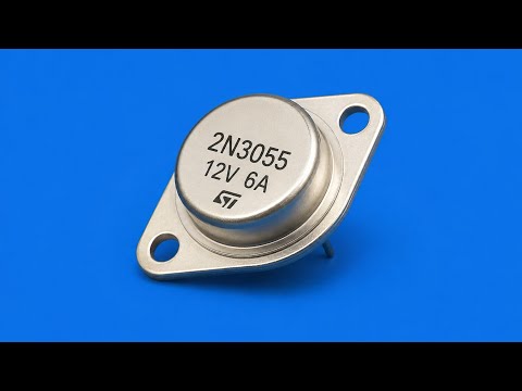
Channel: Variety Creative Channel (149 subscribers)
The 2N3055 is one of the most iconic power transistors in electronics history — a TO-3 packaged NPN workhorse introduced by RCA in the 1960s that still shows up in linear power supplies, audio amplifiers, and hobbyist projects six decades later. This video walks through building a discrete linear voltage regulator that takes a 20–30V input and produces a stable 12V output capable of sourcing up to 6 amps.
What makes this worth watching is the educational value of seeing a pass-transistor regulator built from discrete components rather than dropping in a three-terminal IC like an LM7812. You get to see how a Zener diode establishes the reference voltage, how the 2N3055 acts as the series pass element handling the bulk of the current, and why heatsinking matters when you're dissipating potentially 100+ watts as heat at full load (remember: a linear regulator burns the voltage difference times the current).
This is a great teaching circuit because it demystifies what's actually happening inside a linear regulator chip. Once you understand this topology, you'll have a much better intuition for efficiency tradeoffs, thermal design, and why switching regulators eventually displaced linear designs for high-current applications.
The clickbait emoji in the title is unfortunate, but the underlying content — a classic discrete regulator build — is solid foundational electronics.
Daily YT Engineering
Cantilever Failure Simulation | لماذا فشل الكانتليفير؟ ANSYS Structural Analysis
2026-06-11

Channel: Adham Mohamed (79 subscribers)
This video stands out from the rest of the candidates because it bridges the gap between textbook theory and real-world finite element analysis. Most of the other videos in this batch are board-and-marker lectures about support reactions and shear/moment diagrams — useful, but well-trodden ground. This one opens with a concrete engineering scenario: a cantilever structure that failed due to poor design, and then walks through recreating that failure inside ANSYS.
That format is genuinely instructive. You see why the failure happened (stress concentrations, deflection beyond limits, or material yielding at the fixed support), not just the abstract equations that predict it. Reproducing a failure in simulation is one of the better ways to build intuition for what the math is actually describing — the stress contour plots make invisible forces visible.
From a 79-subscriber channel, the production effort here is also notable: it's a hybrid scenario-plus-tutorial rather than a screen recording with no narrative. For anyone learning FEA, studying for structural exams, or transitioning from hand calculations to software-based analysis, watching a known-failure case modeled end-to-end is more valuable than another worked example of a healthy beam.
Note: the video appears to be partially in Arabic based on the title, so non-Arabic speakers may need to rely on the visual ANSYS workflow.
Daily YT Maker
V-Body Electric Guitar Project Part 1
2026-06-11

Channel: Ronnie Media (35 subscribers)
This is a tiny channel (just 35 subscribers) taking on an ambitious multi-part build: a custom V-body electric guitar starting from a raw alder blank on a CNC mill. Part 1 focuses specifically on CNC milling the body blank, which is where a surprising amount of luthiery knowledge intersects with CAM strategy.
What makes guitar bodies a genuinely educational CNC subject: you're dealing with a soft tonewood that tears out easily, complex contoured surfaces (the belly cut, forearm bevel, pickup cavity pockets at different depths), and tight tolerances on neck pocket geometry that affect playability. Watching how a maker fixtures the blank, chooses bits for roughing versus finishing passes, and handles the transition between flat pocketing and 3D surfacing tells you a lot about real-world CNC workflow.
Alder is also a smart choice to follow along with — it's the classic Fender body wood, forgiving to machine, and visually shows tool marks clearly so you can see where the roughing toolpath ends and the finishing pass begins. For anyone considering instrument building or just looking to level up their CNC project ambitions, this kind of from-scratch build series from a small creator is exactly the type of content worth supporting early.
Daily YT Welding
Arruela de MADEIRA no mini torno #minitorno #usinagem #tornomecanico
2026-06-11

Channel: Henry Guido (4 subscribers)
Honest disclaimer: this week's crop is mostly hashtag spam and Shorts, so the bar is low — but Henry Guido's video genuinely earns its spot. He designed and fabricated his own mini metal lathe from scratch, and this clip puts it through a real test cut: turning a wooden washer to check concentricity, surface finish, and tool behavior on a softer workpiece.
Why wood on a metal lathe is actually a smart shakedown test: wood is forgiving of feed-rate mistakes but ruthlessly exposes spindle runout, headstock alignment, and chatter. If your homemade lathe leaves a clean, concentric finish on end-grain wood, the geometry is solid. If it tears or leaves spiral marks, you've got a tuning problem to chase down.
The description notes the finish came out well, which is meaningful coming from a builder-operator who knows exactly what tolerances went into the machine. For anyone interested in shop-built tooling, the workflow of "build it, then prove it with progressively harder cuts," or just the satisfying physics of a small lathe doing its job, this is a quiet, substantive watch from a 4-subscriber channel that deserves more eyes.
