Daily Digest — 2026-06-12
26 newsletters today.
In this digest
- Abandoned Futures — The Rotodyne: The 190-MPH Compound Helicopter That Could Have Owned City-Center Aviation and Got Killed by a Noise Complaint
- ArXiv Paper Digest — The End of Code Review: Coding Agents Supersede Human Inspection
- Daily Automotive Engines — Turbocharger Compressor Wheel Nut Torque and Stretch
- Daily Debugging Puzzle — Python's NaN-in-Set Trap: The Dedup That Passes Tests and Fails in Production
- Daily Digital Circuits — Store Buffers and Memory Ordering: How Hardware Hides Write Latency at the Cost of Sequential Consistency
- Daily Electrical Circuits — Soft-Start Circuits: Ramping Up Power Supplies Gracefully
- Daily Engineering Lesson — Additive Manufacturing: Why 3D Printing Changed What Engineers Can Design
- Forgotten Books — The Lost Art of the Toilet Soap: When Cleansing Was Chemistry
- Forgotten Darkroom — The Chemistry Textbook Caught Mid-Revolution: When Photographers Worked With Two Incompatible Atomic Theories
- Forgotten Patent — Dennis Gabor's "Wavefront Reconstruction": The 1947 Patent That Invented Holography 13 Years Before the Laser — and Now Hides Inside Every AR Headset and Banknote
- Daily GitHub Zero Stars — KyleSFerguson/zotero-scholar-checker
- Daily Hardware Architecture — The Replacement Policy's Scan-Resistance Problem: Why LRU Falls Apart on Streaming Workloads
- Hacker News Deep Cuts — I am (not) a Failure: Lessons Learned From 6&1/2 Failed Startup Attempts (2025)
- HN Jobs Teardown — Datadog: What Their Hiring Reveals
- Daily Low-Level Programming — The Architectural Event Trace (Intel AET): How the CPU Records Microarchitectural State Without Probes
- RFC Deep Dive — RFC 8952: Captive Portal Architecture
- Stack Overflow Unanswered — How to do an interface between the PC counter and synchronous instruction cache in a 5-stage pipeline
- Daily Software Engineering — The Causal Consistency Pattern: Preserving Cause-and-Effect Order Across Replicas
- Tool Nobody Knows — ttyplot: Real-Time Plotting When You Refuse to Leave the Terminal
- What If Engineering — What If We Built a 100-Story Vertical Farm That Fed an Entire City?
- Wikipedia Rabbit Hole — Tribotronics
- Daily YT Documentary — Granada 4K - The LAST MUSLIM City of Spain - Mini Documentary
- Daily YT Electronics — 12V Plug-In Power Supply Review & Test | Budget Power Adapter Worth Buying?
- Daily YT Engineering — Lec03: Thermodynamic Analysis of Vapor Power Cycle #swayamprabha
- Daily YT Maker — DIY French Cleat Belt Sander Holder | Free CNC Files & Workshop Organization
- Daily YT Welding — Which Welding Type Do You Actually Need? tips quick choose types of welding and their applications
Abandoned Futures
The Rotodyne: The 190-MPH Compound Helicopter That Could Have Owned City-Center Aviation and Got Killed by a Noise Complaint
2026-06-12
On 5 January 1959, a fat-bellied British aircraft called the Fairey Rotodyne set a world speed record for convertiplanes: 190.9 mph over a 100-km closed circuit. It took off vertically from a London heliport, cruised like an airliner, and landed vertically again. It carried 40 passengers. It worked. Six years later, the British government cancelled it, the tooling was scrapped, and the only prototype was broken up for spares.
The Rotodyne was a compound gyroplane, and the engineering is still elegant. Two Napier Eland turboprops on stub wings provided forward thrust. For takeoff and landing, compressed air was bled from the engines, ducted up the rotor mast, out through the four hollow rotor blades, and burned with fuel in tip-jets at each blade end. The rotor was driven from the tips, not the hub — which meant no torque reaction, so no tail rotor was needed. Once airborne and moving forward, the tip-jets shut off and the rotor autorotated like a gyrocopter, while the wings and props carried the load. It was a helicopter for hovering and a fixed-wing aircraft for cruising, switching seamlessly between the two.
The performance numbers from 1959 still embarrass modern rotorcraft. The V-22 Osprey, sixty years and roughly $40 billion later, cruises at 275 mph but carries 24 troops. The Rotodyne cruised at 190 mph carrying 40 passengers or 8 tonnes of cargo, with a planned stretched variant ("Type Z") targeting 220 mph and 70 seats. BEA had ordered six. New York Airways wanted five. Kaman in the US had licensed the technology. The Japanese were interested. Then came the noise.
The tip-jets, burning kerosene at the ends of a 90-foot rotor, produced a low-frequency thumping that registered around 96 dB at 600 feet. London residents near Battersea Heliport complained. The Ministry of Aviation, already nervous about subsidising both Westland and Fairey, used noise as the pretext to merge the companies and quietly bury the Rotodyne in February 1962. By then engineers had already reduced tip-jet noise by 10 dB and had a plan to reach 15 dB further reduction with acoustic liners and pulsed combustion. They were never given the chance.
Why 2026 should care:
- eVTOL is rediscovering the same physics. Joby, Archer, and Lilium are all chasing the city-to-airport segment the Rotodyne was sized for — and none can match its payload-per-disc-loading.
- Tip-jet noise is now a solved problem. Modern swirl-stabilised combustors, ceramic acoustic liners, and active noise cancellation can knock 20–25 dB off a tip-jet without losing thrust. The 96 dB figure that killed the Rotodyne would today come in below 75 dB — quieter than a city bus.
- Hydrogen changes the calculus completely. Tip-jets burning gaseous H₂ produce no soot, run cooler, and eliminate the tip-mounted fuel plumbing that was a 1959 maintenance headache. Reaction Engines and ZeroAvia have already demonstrated the combustor scaling.
- The compound gyroplane beats tiltrotors on cost. No tilt mechanism, no synchronising shaft between nacelles, no transition envelope full of dead-man corners. Sikorsky's Raider X and Airbus's RACER are quietly readmitting that Fairey was right.
The Rotodyne wasn't killed by physics. It was killed by a noise problem we now know how to fix, in an industry consolidation that nobody remembers, by a ministry that couldn't see past its own balance sheet.
ArXiv Paper Digest
The End of Code Review: Coding Agents Supersede Human Inspection
2026-06-12
For fifty years, code review has been a near-sacred ritual in software engineering. Since Michael Fagan formalized "code inspection" at IBM in 1976, the workflow has stayed remarkably stable: one engineer writes code, another reads it carefully before it gets merged. The reviewer hunts for bugs, suggests cleaner approaches, asks "did you think about X?", and approves the change. This practice is so embedded that virtually every serious software organization on Earth — from two-person startups to Google — treats it as non-negotiable.
Monperrus argues, provocatively, that this era is ending. His claim: coding agents have crossed a capability threshold where they can do code review better than humans, and the industry should stop pretending otherwise.
The argument hinges on a few observations:
- Agents are tireless and consistent. Human reviewers get fatigued, skim large diffs, and miss issues in unfamiliar parts of the codebase. An LLM-based agent reviews the 800th line of a diff with the same attention as the first.
- Agents can actually run things. A human reviewer typically reads code statically. An agent can execute tests, reproduce bugs, check whether the change actually compiles in edge cases, and run static analyzers — all in seconds.
- Agents have broader context. A reviewer who hasn't touched a module in months has to page it back in. An agent can re-read the entire relevant subsystem on every review.
- The bottleneck has flipped. When agents write most of the code, having humans review every agent-generated PR becomes the slow step — and humans are now the less-capable reviewers in many domains.
Monperrus isn't claiming humans become irrelevant. The shift he describes is more like what happened to compilers: humans no longer hand-check assembly output because the compiler is trusted to do it correctly. Code review, in his framing, becomes an automated quality gate that humans supervise at a meta-level rather than performing line-by-line.
The key insight is uncomfortable: code review's value was never the ritual itself — it was catching defects and maintaining quality. If agents catch more defects faster and cheaper, then defending human review on principle is mistaking the tool for the goal. The same logic that retired punch cards, manual memory management, and hand-rolled assembly is now coming for the pull request comment thread.
Whether or not you buy the strong version of the claim, the paper forces a question every engineering org will face in the next year: what is human code review actually for, once agents can do it competently?
Daily Automotive Engines
Turbocharger Compressor Wheel Nut Torque and Stretch
2026-06-12
The compressor wheel nut is the single fastener holding a 200,000+ RPM aluminum wheel onto the turbo shaft. Get the torque wrong and you'll either spin the wheel off into the housing or stretch the shaft until it snaps. This tiny nut — often just M6 or M7 — carries one of the most punishing duty cycles in the entire engine.
Why it's so critical: At full boost, the compressor wheel sees three simultaneous loads: centrifugal hoop stress trying to fly the blades outward, axial thrust from compressing air, and bending moments from gas pulsations. The nut must clamp the wheel hard enough that the wheel and shaft act as one rigid body — any micro-slip means fretting, imbalance, and eventual fatigue failure.
The stretch principle: Modern turbo nuts are torqued into the elastic stretch zone, just like rod bolts. The shaft itself is necked down under the nut so it stretches predictably. Garrett's GT/GTX series typically calls for torque-plus-angle: snug to ~25 in-lb, then rotate exactly 90° more. This achieves roughly 0.004–0.006" of shaft stretch, which corresponds to about 2,500 lbs of clamp load on a GT3582R-sized shaft.
Left-hand threads — almost always: Because the turbo spins clockwise viewed from the compressor end, a right-hand thread would loosen under rotational inertia during spool. Nearly every modern turbo uses left-hand threads on the compressor nut. Get this wrong during a rebuild and you'll snap the shaft trying to "tighten" it.
Real-world example: Borg Warner EFR series uses a titanium compressor nut with a published spec of 18 in-lb + 90°. A common rebuild failure mode: a shop uses an impact gun, blows past the angle spec, yields the shaft past its elastic limit, and the turbo grenades at 22 psi three weeks later. Compressor wheel found embedded in the intercooler core.
Rule of thumb for stretch torque:
- Final clamp load ≈ 60–70% of the shaft's yield strength
- For a 7mm necked shaft (~38 mm² cross-section) in 4340 steel: yield ≈ 6,800 lbs, so target clamp ≈ 4,500 lbs
- Shaft stretch = (Load × Length) / (Area × Modulus) — for steel, roughly 0.001" per 1,500 lbs per inch of necked length
Reuse warning: Stretch fasteners are technically single-use. Most turbo rebuilders replace the nut every time the wheel comes off, because re-yielding a previously stretched shaft section drops clamp load by 15–20% on the second torque cycle.
Daily Debugging Puzzle
Python's NaN-in-Set Trap: The Dedup That Passes Tests and Fails in Production
2026-06-12
This sensor pipeline deduplicates measurement readings while preserving order. The unit tests pass, code review approves it, and it ships. A week later, downstream consumers complain that error sentinels are appearing multiple times in the "deduplicated" output.
import json

def deduplicate(values):
    """Remove duplicate measurements, preserving first-seen order."""
    seen = set()
    unique = []
    for v in values:
        if v not in seen:
            seen.add(v)
            unique.append(v)
    return unique

# --- unit test (passes) ---
NAN = float('nan')
result = deduplicate([1.0, NAN, 2.0, NAN, 3.0])
assert result == [1.0, NAN, 2.0, 3.0]    # ✓ passes

# --- production code path ---
payload = '{"readings": [1.0, NaN, 2.0, NaN, 3.0]}'
readings = json.loads(payload)["readings"]
print(deduplicate(readings))
# Expected: [1.0, nan, 2.0, 3.0]
# Actual:   [1.0, nan, 2.0, nan, 3.0]
The Bug
Two facts collide here, both individually well-known, but together devastating:
- IEEE 754 says
NaN != NaN. By design, no NaN compares equal to anything, including itself. - CPython's set and dict membership tests use identity-then-equality. The membership check is effectively
x is candidate or x == candidate. The identity shortcut exists for speed and to make weird objects (like NaN) at least seem well-behaved in collections.
In the unit test, every NAN in the list is literally the same Python object (id(NAN) is constant). When the loop hits the second NAN, the identity check v is seen_element returns True, and it's correctly skipped. The assertion also passes for the same reason — list equality is element-wise with the same identity-first rule.
In production, json.loads manufactures a fresh float('nan') object for every NaN token. Now each NaN in the list is a different object: identity fails, equality fails (NaN != NaN), and the "dedup" passes every NaN straight through. The deeper the pipeline, the worse it gets — every float(), numpy conversion, or arithmetic result that yields NaN produces a brand-new object.
The trap is especially nasty because the test looks like it covers the case. Reviewers see a NaN in the input and a deduplicated NaN in the expected output, and conclude the function handles NaN. It doesn't — it handles shared-identity NaN, which is an artifact of how the test was written, not a property of the data.
The Fix
Canonicalize NaN explicitly. Either drop it, or replace every NaN with a single sentinel before the set check:
import math

def deduplicate(values):
    seen = set()
    unique = []
    nan_seen = False
    for v in values:
        if isinstance(v, float) and math.isnan(v):
            if nan_seen:
                continue
            nan_seen = True
            unique.append(v)
        elif v not in seen:
            seen.add(v)
            unique.append(v)
    return unique
The same pattern bites dict keys, Counter, functools.lru_cache with float arguments, and anywhere "value equality" is silently doing identity equality for you. If your data can contain NaN, write a test where the NaNs come from different sources — parsing, arithmetic, conversion — not a shared module-level constant.
Daily Digital Circuits
Store Buffers and Memory Ordering: How Hardware Hides Write Latency at the Cost of Sequential Consistency
2026-06-12
When a CPU executes a store instruction, the data doesn't go straight to the cache. It lands in a store buffer — a small FIFO of pending writes sitting between the execution units and the L1 data cache. The core continues executing subsequent instructions while the buffer drains in the background. This is why your write to memory looks like a 1-cycle operation even though committing it to L1 might take 3–5 cycles, and to L2 might take 15.
The store buffer solves a real problem: stores are slow compared to loads. A store needs to acquire the cache line in Modified state (MESI), which may require an invalidation broadcast to other cores. Without a buffer, every store stalls the pipeline until the line arrives. With a buffer, the core fires-and-forgets — the store retires architecturally while the buffer entry waits for the line.
But here's where it gets nasty: store-to-load forwarding. If the core executes a load to the same address as a buffered store, it must read from the buffer, not the cache. This requires associative address comparison on every load — the buffer is essentially a small CAM. Partial overlaps (4-byte store, 8-byte load) cause a store forwarding stall, often 10–15 cycles, because the hardware gives up and waits for the store to commit.
The deeper consequence is memory ordering relaxation. On x86 (TSO — Total Store Order), stores in the buffer are visible to the issuing core via forwarding but invisible to other cores until they drain. This means thread A can see its own store immediately, while thread B still sees the old value. The classic Dekker's algorithm failure mode:
- Core 0:
store X=1; load Y - Core 1:
store Y=1; load X - Both stores sit in their respective buffers. Both loads bypass into cache and read 0.
- Both cores observe the other's variable as still zero — a state impossible under sequential consistency.
This is why MFENCE (x86) or dmb ish (ARM) exist: they drain the store buffer before allowing subsequent loads. A typical x86 MFENCE costs 20–40 cycles because it must wait for every buffered store to commit to L1.
Rule of thumb: store buffer depth is roughly 50–80 entries on modern x86 (Intel Skylake: 56; AMD Zen 4: 64). If your code stores faster than the L1 can absorb (~1 store/cycle sustained), the buffer fills, and the pipeline stalls on the next store. Loop unrolling that emits 4+ stores per iteration often hits this wall before it hits any arithmetic limit.
Daily Electrical Circuits
Soft-Start Circuits: Ramping Up Power Supplies Gracefully
2026-06-12
When a switching power supply turns on, the output capacitor looks like a short circuit. The control loop slams the duty cycle to maximum trying to regulate, and the inductor current spikes — sometimes tripping overcurrent protection, saturating the transformer, or stressing the input bulk caps. Soft-start circuits solve this by gradually ramping the reference voltage (or duty cycle limit) over milliseconds instead of microseconds, letting the output charge in a controlled fashion.
The basic mechanism: most modern controllers (LM5085, TPS54x, UCC28x) expose an SS pin. You hang a capacitor from SS to ground; an internal current source (typically 1–10 µA) charges it linearly. The error amplifier's reference is clamped to whichever is lower — the true bandgap reference or the SS voltage. As C_ss charges, the effective reference ramps from 0 V up to the bandgap, dragging the output up with it.
Sizing the capacitor: the ramp time is
- tss = (C_ss × V_ref) / I_ss
For a controller with V_ref = 0.8 V and I_ss = 5 µA, a 10 nF cap gives t_ss = (10 nF × 0.8 V) / 5 µA = 1.6 ms. Rule of thumb: aim for 1–10 ms on most converters. Too fast and you defeat the purpose; too slow and the supply may not be ready when downstream rails expect it.
Real-world example: a 12 V → 3.3 V buck powering an FPGA with 470 µF of output bulk capacitance. Without soft-start, charging that to 3.3 V instantly requires I = C·dV/dt — at 10 µs ramp, that's 155 A of inductor current. The MOSFET cooks, OCP trips, and the supply hiccups indefinitely. With a 5 ms soft-start, peak charging current drops to 310 mA — well within normal operating range. The FPGA's POR circuit sees a clean monotonic rise and boots reliably.
DIY soft-start without a dedicated pin: for a linear regulator like an LM317, put an RC network on ADJ. A 10 µF cap from ADJ to ground with the normal feedback resistors gives a ramp time of roughly R2 × C_ss. For a brute-force solution on any supply, an N-channel MOSFET inrush limiter with a gate-RC delay works — the gate charges slowly, VGS traverses the linear region, and the MOSFET behaves momentarily as a variable resistor.
Pitfalls: a soft-start that's slower than your undervoltage lockout (UVLO) recovery causes restart loops. And don't forget that soft-start only controls startup — it doesn't help with load transients or recovery from a fault.
Daily Engineering Lesson
Additive Manufacturing: Why 3D Printing Changed What Engineers Can Design
2026-06-12
Additive manufacturing (AM) builds parts layer by layer from a digital model, the opposite of subtractive processes that carve away material. The key insight: geometric complexity is free. A lattice-filled bracket costs the same to print as a solid one — sometimes less, because it uses less material and prints faster.
The major metal AM processes:
- Powder Bed Fusion (PBF) — A laser or electron beam melts metal powder one layer at a time. Selective Laser Melting (SLM) and Electron Beam Melting (EBM) dominate aerospace and medical. Layer thickness: 20-100 μm.
- Directed Energy Deposition (DED) — Powder or wire fed into a melt pool. Used for large parts and repair (turbine blade tips, worn shafts). Lower resolution, higher deposition rate.
- Binder Jetting — Inkjet print binder onto powder, then sinter. Cheaper, faster, but parts shrink ~20% during sintering — dimensional control is harder.
Polymer AM is dominated by FDM (extruded filament, cheap and ubiquitous), SLA/DLP (UV-cured resin, smooth surfaces), and SLS (laser-sintered nylon powder, strong functional parts).
Real-world example: GE's LEAP engine fuel nozzle. The original design had 20 separately-machined pieces brazed together. The 3D-printed version is a single piece, 25% lighter, and 5× more durable. GE prints over 30,000 of them per year using SLM. The redesigned internal cooling passages — impossible to machine — actually improve combustion efficiency.
Design rules of thumb for metal PBF:
- Overhangs over 45° from vertical need support structures. Self-supporting angles save post-processing time.
- Minimum wall thickness ~0.4 mm; minimum hole diameter ~0.5 mm (smaller holes need drilling).
- Build orientation matters — tensile strength along the build direction (Z) is typically 10-20% lower than in-plane (XY), and surface finish is roughest on downward-facing surfaces.
- Plan for post-processing: stress relief heat treatment, support removal, HIP for porosity, machining of critical surfaces. The "as-printed" part is rarely the finished part.
Cost rule of thumb: Metal AM makes sense when part complexity, low volume (under ~1000/year), or weight savings justify the cost — typically $50-500 per cubic inch of metal printed. Below that volume and complexity, machining wins. Above it, casting plus machining usually still beats AM on cost alone.
The biggest mindset shift: stop designing parts that could be machined and then printing them. Topology optimization, internal channels, integrated assemblies, and biomimetic lattices are where AM earns its keep.
Forgotten Books
The Lost Art of the Toilet Soap: When Cleansing Was Chemistry
2026-06-12
Book: A Practical Handbook Of The Manufacture Of Hard And Soft Soaps, Toilet Soaps by Watt, Alexander (1901)
Read it: Internet Archive
The excerpt I recovered from this 1901 volume is largely a casualty of optical character recognition gone sideways — the digitized pages read as a fog of broken Devanagari fragments and scattered Roman letters. But within the wreckage, the structure of an old publisher's advertisement leaf emerges, hawking companion volumes on "Practical Treatises" for tradesmen, and praising one work as:
"A book of value to be kept his bench by every... worker in metals or alloys."
This was the world Alexander Watt wrote for: the bench worker, the small manufacturer, the village chandler. Watt was a prolific Victorian industrial chemist whose handbooks — on electroplating, leather-dressing, and soap — assumed a reader who would actually make the thing, not just buy it.
The forgotten knowledge here isn't a single recipe. It's the entire premise that a literate adult could and should manufacture their own soap, distinguishing scientifically between hard soap (sodium-based, for laundry), soft soap (potassium-based, for industry and medicine), and the painstaking "toilet soap" — the perfumed, milled, skin-conditioning bar that required boiling, salting-out, crutching with essential oils, and careful re-melting.
Watt's contemporaries took for granted things our generation has comprehensively forgotten:
- That soap is just saponified fat. Any animal tallow or vegetable oil plus an alkali (lye from wood ashes, in a pinch) yields soap. The chemistry is grade-school simple — yet most modern adults could not produce a bar to save their lives.
- That "toilet" originally meant grooming, not plumbing. A toilet soap was a personal-care soap. The handbook devoted entire chapters to coloring agents, perfumes, and the "transparent" glycerine soaps that Pears advertised so aggressively in Watt's day.
- That soft potassium soap had medicinal uses. Watt-era pharmacopoeias prescribed soft soap as a vehicle for sulfur, tar, and mercury treatments — a tradition that survives only in obscure dermatological preparations like sapo kalinus.
Is any of this still useful? Surprisingly, yes. The home soap-making revival on social media — the cold-process YouTube tutorials, the Etsy lavender-tallow bars — is essentially the rediscovery of chapter three of Watt's handbook, often by people who don't know it exists. And the dermatology literature has, in the last decade, swung back toward Watt's view that industrial detergents (sodium lauryl sulfate, etc.) are harsher on the skin barrier than traditional saponified-fat soap. The "syndet bar" boom and the eczema-driven return to old-fashioned bar soap are, in effect, Watt being right again 125 years later.
The deepest forgotten thing is not a recipe but a stance: that the contents of your washbasin should be intelligible to you, traceable to a fat and an alkali you could name. We outsourced that knowledge to Procter & Gamble around 1890 and never asked for it back.
Forgotten Darkroom
The Chemistry Textbook Caught Mid-Revolution: When Photographers Worked With Two Incompatible Atomic Theories
2026-06-12
Book: A manual of photographic chemistry : theoretical and practical by Hardwich, T. Frederick (1864)
Read it: Internet Archive
Buried in the preface to the seventh edition of Hardwich's Manual of Photographic Chemistry, the editors George Dawson and Edward Hadow — both of King's College, London — make a startling admission about the state of chemistry in 1864:
"Although this portion of the Book has been in a great measure re-written, old-fashioned definitions of Acids and Salts, and modes of representing chemical changes, have been retained, since later and more exact views could hardly be introduced without the frequent employment of new terms, which seem out of place in a Manual treating only of what is theoretical for practical ends. Those Atomic Weights are given which accord with the ordinary chemical names familiar to Photographers."
Translation: we know the new chemistry is better, but our readers learned the old notation, so we're sticking with it.
This is a remarkable historical fossil. The book was written at exactly the moment chemistry was tearing itself apart. The Karlsruhe Congress of 1860 — just four years earlier — had finally settled the long battle over atomic weights, with Stanislao Cannizzaro convincing a generation of chemists that Avogadro's hypothesis was correct and that water was H₂O, not HO. Before Karlsruhe, chemists couldn't even agree whether the atomic weight of oxygen was 8 or 16. Different textbooks used different formulas for the same compounds.
Hardwich's editors are telling us, in dry Victorian prose, that working photographers in the 1860s were still using the pre-Karlsruhe equivalent-weight system — the system where silver nitrate might be written as AgO,NO₅ rather than AgNO₃ — because that was the language printed on their chemical bottles and in their darkroom recipes.
What's lost to modern readers isn't a recipe or a remedy. It's the memory that modern chemistry is much younger than you think. The atomic theory you learned in high school — the one where every element has a single, agreed-upon atomic weight, and every compound has a single, unambiguous formula — was barely cementing itself when American Civil War photographers were coating wet collodion plates at Antietam.
The editors' choice has a modern echo. Consider:
- Python 2 vs Python 3: a community split over notation that persisted for over a decade because practitioners couldn't afford to rewrite their working code.
- Imperial vs metric units in American engineering: NASA still loses spacecraft to this.
- Pre-SI electrical units: the abampere, statvolt, and gauss lingered in physics textbooks well into the 1980s.
Hardwich's preface captures a universal pattern: a working profession will keep using deprecated notation long after academics have moved on, because the cost of relearning exceeds the benefit of precision. The photographers of 1864 weren't ignorant — they had made a rational economic choice. Their chemistry worked. Their pictures came out.
The "wrong" notation made beautiful tintypes.
Forgotten Patent
Dennis Gabor's "Wavefront Reconstruction": The 1947 Patent That Invented Holography 13 Years Before the Laser — and Now Hides Inside Every AR Headset and Banknote
2026-06-12
In the winter of 1947, a Hungarian-British engineer at British Thomson-Houston in Rugby was trying to fix the electron microscope. Dennis Gabor thought the resolution problem wasn't optical — it was informational. Lenses were throwing away half the data in a wavefront: the phase. Photographic plates recorded brightness but not the angle at which light arrived. So Gabor proposed something audacious: record the interference pattern between a reference wave and a scattered object wave, and the plate would store the entire wavefront. Shine the reference wave back through the plate, and the original 3D scene would reconstruct itself in mid-air.
He filed British Patent 685,286 on December 17, 1947, followed by US Patent 2,770,166 ("Improvements in and Relating to Microscopy"), granted November 1956. He coined the word hologram from the Greek holos — "whole" — because it captured the whole light field.
There was one catastrophic problem: coherent light didn't exist yet. To make a clean interference pattern, you need a source where every photon marches in lockstep. Gabor's best option was a high-pressure mercury arc lamp filtered through a pinhole, then through a monochromator. The coherence length was about 0.1 mm. His holograms were murky, ghostly, and suffered from a "twin image" problem where the real and virtual reconstructions sat on top of each other. The technique was a theoretical triumph that produced almost unusable images.
Then in 1960 Theodore Maiman fired the first ruby laser. Suddenly coherent light was cheap, bright, and continuous. In 1962, Emmett Leith and Juris Upatnieks at the University of Michigan dusted off Gabor's papers, added an off-axis reference beam to kill the twin image, and produced the first clean laser holograms — a toy train, a chess set — that looked like solid objects floating in glass. Gabor won the 1971 Nobel Prize in Physics, having waited 24 years for the rest of physics to catch up to his patent.
The modern footprint is enormous and mostly invisible:
- AR and mixed-reality headsets — Microsoft HoloLens 2, Magic Leap 2, and Apple Vision Pro all use holographic optical elements or surface-relief gratings in their waveguides. These are direct descendants of Gabor's wavefront-reconstruction principle, etched in nanometer-thick polymers.
- Anti-counterfeiting — the rainbow holograms on every credit card, passport, and banknote use embossed surface holograms invented by Stephen Benton at Polaroid in 1968, building on Gabor.
- Holographic data storage — Akonia Holographics (acquired by Apple in 2018) and Microsoft's Project HSD store terabytes per square centimeter by writing thousands of overlapping holograms into photopolymer.
- Optical neural networks — companies like Lightmatter and Lightelligence use computer-generated holograms as the diffractive layers that perform matrix multiplications at the speed of light.
- EUV lithography — ASML's chip-making machines use phase-shifting masks that are, mathematically, holograms designed to sculpt the wavefront that exposes silicon.
Gabor's patent is also a clean case study in the missing prerequisite problem of invention. The math, the optics, and the photographic chemistry were all available in 1947. The one thing missing — a source of coherent light — wouldn't exist for 13 more years. Gabor patented a complete idea that the universe could not yet execute. The patent itself describes the laser-era technique perfectly; he just had to wait for someone to invent the right lamp.
Daily GitHub Zero Stars
KyleSFerguson/zotero-scholar-checker
2026-06-12
Language: JavaScript
Link: https://github.com/KyleSFerguson/zotero-scholar-checker
This is one of those small, sharply-scoped browser extensions that solves a real workflow papercut for a very specific audience — and that's exactly why it caught my eye. zotero-scholar-checker is a Chrome extension that bridges your Zotero library with Google Scholar search results, surfacing your reading status and PDF tags directly on the Scholar results page.
What it does:
- Queries your local Zotero library while you browse Google Scholar
- Annotates each search result with whether you've already saved it
- Surfaces your existing PDF tags inline, so you can see at a glance how a paper fits into your prior reading
- Eliminates the constant alt-tabbing between Scholar and your reference manager
Why it's interesting: Most academic-workflow tools are either heavyweight cloud platforms or stale Firefox extensions abandoned circa 2018. A modern, focused Chrome extension that talks to a local Zotero instance is genuinely useful — and it's the kind of project that a researcher writes for themselves first and shares second. That tends to produce better software than tools designed by committee. The fact that it lives in the browser, rather than as another Zotero plugin, also means it intercepts the discovery step (Scholar) rather than waiting for you to remember to check Zotero after the fact.
Who would benefit:
- Graduate students and PhD researchers drowning in literature reviews where the same paper surfaces across multiple searches
- Academics doing systematic reviews who need to track which references have already been triaged
- Anyone using Zotero's tagging system seriously — the surfaced-tags feature rewards disciplined tagging habits
For a zero-star repo pushed today, this is the kind of niche utility that could quietly become indispensable to its small audience. Worth a star if you live in Scholar.
Daily Hardware Architecture
The Replacement Policy's Scan-Resistance Problem: Why LRU Falls Apart on Streaming Workloads
2026-06-12
LRU (Least Recently Used) sounds like the obvious cache replacement policy: throw out the line you haven't touched in the longest time. It works beautifully when your working set fits in cache. It catastrophically falls apart the moment your workload scans — touches a large array once, then moves on.
Here's the failure mode: imagine an L2 cache that holds 16 MB. Your hot working set is 12 MB and benefits enormously from caching. Then your program does memcpy over a 64 MB buffer. Every line in that 64 MB buffer enters L2, marked as "most recently used." LRU dutifully evicts your hot 12 MB to make room for streaming data that will never be touched again. After the memcpy, your hot data is gone, and the streaming data sits there cold until it ages out. This is called cache pollution, and it's why pure LRU lost its crown.
The fix is scan-resistance: don't immediately promote new lines to "most recently used." Instead, insert them near the eviction end of the LRU stack, and only promote them if they get a second hit. Lines that are touched once and never again get evicted quickly. Lines that prove themselves get protected. This is the core idea behind RRIP (Re-Reference Interval Prediction) and Intel's DRRIP, which ships in modern Xeon L3 caches.
In RRIP, each line gets a 2-bit counter (the "re-reference prediction value," or RRPV):
- 0 = expected to be reused immediately
- 3 = expected to be useless soon (evict next)
New lines are inserted with RRPV=2 — not RRPV=0. They have to earn promotion to RRPV=0 through a hit. On eviction, the cache scans for any line with RRPV=3; if none exists, it increments all RRPVs and tries again. This means scanned-once lines get evicted within roughly two passes, while reused lines stay protected.
Rule of thumb: If your workload's footprint exceeds your last-level cache by 2× or more and you see no reuse within that pass, you're paying for cache pollution on LRU. Use non-temporal stores (MOVNTDQ, vmovntps) or prefetchnta to bypass the cache entirely — you're telling the hardware "don't bother caching this, I won't be back." On modern Intel chips with DRRIP, the policy itself handles this gracefully, but explicit hints still help.
The deeper lesson: the "obvious" caching policy assumes recency predicts reuse. For scans, that assumption is exactly backwards — recency predicts uselessness.
Hacker News Deep Cuts
I am (not) a Failure: Lessons Learned From 6&1/2 Failed Startup Attempts (2025)
2026-06-12
Link: http://blog.rongarret.info/2025/01/i-am-not-failure-lessons-learned-from.html
HN Discussion: 1 points, 0 comments
Ron Garret is one of those names that should perk up the ears of anyone who's been around the Lisp world or NASA's deep-space program. He was the lead programmer for the Remote Agent that flew on Deep Space 1 — the first AI to autonomously command a spacecraft — and a longtime Googler back when Google was small. He's also written one of the more honest reflections on startup life you'll find on the open web.
The premise of this post is unusual: rather than the typical "five lessons from my successful exit" genre, Garret walks through six and a half failed attempts at building a company. The "half" alone is intriguing — it suggests the kind of granular honesty that survivor-bias-heavy startup writing rarely musters.
Why this deserves more attention than a single upvote:
- Selection bias correction. The startup canon is dominated by founders who won. Reading someone who tried repeatedly and didn't break through — but who is also clearly technically formidable — is genuinely rare and useful signal.
- Credibility. Garret isn't writing as a perpetual aspirant. He's a serious engineer with a real track record at NASA JPL and early Google. When he says "this is what I got wrong," there's no pretense to defend.
- Title framing. The "(not)" in "I am (not) a Failure" hints that the post is wrestling with how we define success in a culture that conflates outcome with merit — a topic the HN crowd argues about constantly without much nuance.
For technical readers, the value here is twofold. First, it's a reality check on the founder mythology: even with strong engineering chops and the right networks, the modal outcome is failure, and failure has texture worth studying. Second, Garret has historically been a thoughtful writer on why technically excellent things don't always win — a lesson that translates beyond startups into open source, internal tools, and career strategy.
The post also dates back to early 2025 but is being resurfaced now, which usually means someone found it durable enough to share a year later. That's a stronger signal than most front-page churn.
HN Jobs Teardown
Datadog: What Their Hiring Reveals
2026-06-12
Source: HN Who is Hiring
Posted by: datadogtr
Datadog's posting (ID 22668236) is a masterclass in confident understatement. In a few sentences, they tell you exactly how they win: "We build our own tsdb, distributed tracing tools, cutting edge visualizations." That single line reveals more strategy than most companies' entire careers page.
The stack tells the story:
Go, Python, Java, React— pragmatic polyglot, not religious about one languagek8s, multi-region, multi-cloud— they live the same infrastructure pain their customers do- Custom TSDB — the big tell. They didn't pick InfluxDB or Prometheus's storage. At "trillions of events per day," off-the-shelf time-series databases hit physics walls. Building your own tsdb is a multi-year, multi-team commitment that becomes a moat competitors can't cross without rewriting from scratch.
What the posting reveals about stage and direction:
Datadog isn't hiring for a feature — they're hiring for scale. The "trillions of events per day" framing is a recruiting filter: they want engineers who think about back-pressure, sharding, and tail latency, not CRUD apps. The Boston/NYC/Paris + REMOTE footprint signals a company that's already past the "everyone in one room" stage and has working distributed engineering culture. Remote-friendly in 2020 was still uncommon for infrastructure companies; Datadog leaning into it suggests they'd rather hire the best systems people anywhere than fight over Bay Area talent.
The "customers just like us" line is the most strategically loaded sentence in the post. It's dogfooding as a recruiting pitch — and a competitive moat. Their engineers ARE the buyer persona. They don't need user research; they have on-call rotations.
Green flags:
- Specific technical claims (trillions of events) rather than vague "scale" hand-waving
- Honest about regions and stack — no buzzword soup
- Single short link, no recruiter funnel chaos
Red flags (mild):
- Generic "Software Engineers" title — no level, no team. Likely a high-volume req that funnels into specific teams post-interview, which can mean candidates get bounced between groups.
- No mention of compensation philosophy, equity refresh, or what "growing fast" means for individual scope.
Daily Low-Level Programming
The Architectural Event Trace (Intel AET): How the CPU Records Microarchitectural State Without Probes
2026-06-12
Intel Processor Trace records which branches you took, but it can't tell you why the pipeline stalled. To answer that, recent Intel server parts ship Architectural Event Trace (AET) — a debug facility that streams microarchitectural events (cache fills, TLB walks, retirement stalls, uop dispatch) into a memory buffer or out the trace port, with each event timestamped against the core clock.
AET is distinct from the PMU you query with perf. The PMU counts events (e.g., "12,847 L3 misses"). AET logs every individual event with its address, latency, and the instruction pointer that caused it. You stop guessing which load missed — the trace tells you the exact RIP and the cycle it resolved.
- Event source taps: Hardware probes wired into the load-store unit, the L1/L2/L3 interfaces, the TLB walker, and the retirement unit. Each tap emits a 16-byte record when its event fires.
- Trace sink: A ring buffer in DRAM (configured via MSR
IA32_AET_CTL), or routed off-chip via the Direct Connect Interface to a logic analyzer for silicon validation. - Filtering: Per-source masks and address-range filters keep bandwidth manageable — full unfiltered AET can hit 30+ GB/s per core.
- Privilege: AET requires SGX-style attestation or platform debug authorization (closed chassis debug). It is not a Ring 0 facility — even the kernel can't enable it without a signed debug token.
Real-world example: A hyperscaler tracked an intermittent 200μs latency spike in a Redis-style KV cache. PMU counters showed elevated MEM_LOAD_RETIRED.L3_MISS during the spike, but couldn't isolate which load. With AET enabled on a debug-fused validation part, they captured 50ms of full memory-event trace around the spike and discovered a single rare load was hitting a remote NUMA node because a kernel thread had migrated the hash bucket page. Fix: mbind() the page to the local node. PMU alone would have taken weeks of guessing.
Rule of thumb for AET bandwidth: Budget ≈ 1 byte per retired uop per enabled event class. A core retiring 4 uops/cycle at 3 GHz with cache + TLB + retirement events enabled produces roughly 36 GB/s of trace data. Your DRAM ring buffer fills in microseconds — always filter by address range or sample rate, never trace unbounded.
RFC Deep Dive
RFC 8952: Captive Portal Architecture
2026-06-12
Everyone has met a captive portal: the hotel Wi-Fi sign-in page, the airport "accept terms" form, the coffee shop voucher screen. For about two decades, captive portals operated entirely outside the standards stack — a tower of hacks that violated nearly every layer of the Internet model. RFC 8952 is the IETF's belated attempt to describe what a proper captive portal should look like, and it sits at the center of a small family of RFCs (8908 for the API, 8910 for the DHCP/RA signaling) that together replace the hacks with a real protocol.
The problem space. Historically, networks trapped unauthenticated clients by:
- Intercepting DNS lookups and returning the portal's IP for every name.
- Transparently proxying TCP/80 and injecting an HTTP
302. - Returning forged HTTP responses to operating-system probe URLs (
captive.apple.com,www.msftncsi.com,connectivitycheck.gstatic.com). - Silently dropping everything else and hoping the user opens a browser.
This worked in 2005. It fails badly in a world of HTTPS-by-default, HSTS, DoH/DoT, QUIC, and background sync. A modern phone wakes up on hotel Wi-Fi, tries a TLS connection to a pinned server, gets a redirect to a self-signed portal, refuses the cert, and the user sees a permanent "no internet" indicator. Meanwhile push notifications, mail fetch, and OS updates all silently fail.
What RFC 8952 actually says. It is an architecture document, not a wire protocol. It identifies three actors — the User Equipment (UE), the Provisioning Service (DHCP/RA), and the Captive Portal API Server — and four behaviors the system must support:
- Signaling: the network tells the client "you are captive" via a standard, trustworthy channel (DHCP option 114, IPv6 RA option, or PvD), not by lying about DNS or HTTP.
- State query: the client asks a JSON API "am I captive, and if so where do I authenticate?" — defined in RFC 8908.
- Enforcement: the gateway still blocks non-authenticated traffic, but it does so honestly (ICMP unreachable, TCP RST, or simply drop) instead of impersonating the destination.
- Notification: the API can return remaining bytes, seconds, or a "session about to expire" hint so the OS can prompt the user proactively.
Key design decisions worth noting. The working group consciously rejected putting portal information inside DNS, because DNSSEC and resolver caching make per-client answers unsafe. They also rejected piggybacking on HTTP because TLS makes HTTP interception strictly worse than useless. The DHCP/RA option carries only a URL (an HTTPS URL, with a real certificate, served by the venue or its hosting provider) — everything else flows over normal TLS.
Why it matters today. iOS 14, macOS Big Sur, Android 11, and Windows 11 all implement RFC 8908/8910. If you maintain a guest network at a hotel, conference, or office, the modern recipe is: hand out DHCP option 114 pointing at an HTTPS endpoint that returns the application/captive+json media type, let the OS surface its own native sign-in sheet, and stop intercepting traffic. The user gets a clean modal instead of broken HTTPS errors; your guests' Apple Watches keep syncing; you stop being blamed for "the Wi-Fi is broken."
The quietly subversive aspect of RFC 8952 is that it formalizes something the IETF spent years refusing to formalize, on the grounds that captive portals are a violation of the end-to-end principle. They are — but pretending they did not exist made the Internet worse, not better. RFC 8952 is what acceptance looks like.
Stack Overflow Unanswered
How to do an interface between the PC counter and synchronous instruction cache in a 5-stage pipeline
2026-06-12
The asker is building a classic 5-stage RISC pipeline (IF/ID/EX/MEM/WB) in VHDL, and it works when the instruction memory behaves as a combinational ROM — present an address, get the instruction back in the same cycle. The trouble starts when they swap in a real block RAM-backed instruction cache. On every FPGA fabric (Xilinx, Intel, Lattice, Gowin), BRAM is fundamentally synchronous: the address is latched on a clock edge, and the data appears on the output port one cycle later. That extra cycle of latency breaks the textbook fetch stage, where the PC and the instruction were assumed to update in lockstep.
What makes this interesting is that the fix isn't just "add a register" — it forces you to re-think where the IF/ID boundary actually lives and how stalls, branches, and resets propagate.
Why it's hard
- The PC and the fetched instruction are now out of phase. When the PC is X on cycle N, the instruction at address X doesn't appear at the BRAM data port until cycle N+1.
- Branches and jumps from EX/MEM need to redirect the PC, and the in-flight fetch (already addressed BRAM last cycle) must be squashed without corrupting the IF/ID register.
- Stalls from load-use hazards have to hold both the PC and the BRAM address constant, otherwise you fetch — and lose — an instruction during the bubble.
- Reset is awkward: BRAM contents around address 0 will be read on the first real cycle, so you typically need to inject a NOP into IF/ID for one cycle after reset.
A direction toward a solution
Treat the BRAM's internal output register as the IF/ID pipeline register itself, rather than adding another flip-flop after it. Then:
- Drive the BRAM address with the next PC (the combinational mux output), not the registered PC. The address-latch flip-flop inside the BRAM is your PC register.
- On a branch mispredict from EX, assert a one-cycle
flush_IFthat forces the instruction emerging from BRAM into a NOP at the ID stage (mux at the IF/ID output, not before it). - On a stall, drive the BRAM's
ena(clock-enable) low so both the address register and the output register hold. This keeps the fetched instruction parked at the ID input until the hazard clears. - Add a 1-bit "valid" flag through IF/ID so post-reset and post-flush cycles inject NOPs cleanly.
Gotchas
- Don't try to "go around" the BRAM with a bypass mux on miss-predict — you can't, the data isn't there yet. You must squash, not substitute.
- Cache misses (not just BRAM latency) need a separate
i_readyhandshake that stalls the whole pipeline; conflating the two will bite you when you add a real cache controller. - Watch for inferred vs. instantiated BRAM: some tools won't infer block RAM unless you use the exact read-first/write-first template, and a registered output adds a second cycle of latency you may not want.
Daily Software Engineering
The Causal Consistency Pattern: Preserving Cause-and-Effect Order Across Replicas
2026-06-12
Eventual consistency lets replicas converge "eventually," but it makes no promises about order. If Alice posts "I lost my cat" and then comments "Found him!", a replica might show the comment before the post. The reply makes no sense without the cause. Causal consistency guarantees that if event A causally precedes event B, every replica observing B has already observed A.
The key word is causally. Concurrent events — writes with no happens-before relationship — can still be seen in any order on different replicas. You're not paying for total ordering; you're only paying to preserve the dependencies that actually matter.
How it works under the hood: each write carries a dependency set — a summary of the writes its author had seen at the time of writing. A replica receiving a write checks its local state against that dependency set. If anything is missing, the write is buffered until the missing dependencies arrive. Vector clocks or version vectors are the usual encoding.
Real-world example: Facebook's TAO and many comment systems use causal consistency. When you reply to a comment, your reply carries metadata saying "I saw comment #4823." A read replica that hasn't yet received comment #4823 will delay showing your reply (or fetch the parent) rather than display an orphaned response. The same principle drives collaborative editors like Google Docs — your keystrokes carry causal metadata so peers never apply your edits before the prior context they depended on.
What it does NOT give you:
- Concurrent writes from independent users may be ordered differently on different replicas — that's fine, they had no causal link.
- It doesn't prevent lost updates on concurrent writes to the same key; you still need conflict resolution (CRDTs, last-write-wins, application merge).
- It doesn't give you linearizability — a read might miss a write that finished a microsecond ago on another replica, as long as you didn't depend on it.
Rule of thumb: if your application has conversations — replies, threads, dependent edits, "after I did X, do Y" workflows — you need at least causal consistency. If every write is independent (telemetry, sensor data, like-counts), eventual is enough. The cost gap is roughly 2-4x metadata overhead per write for vector clocks versus plain timestamps, but it's still cheaper and more available than strong consistency.
Causal is the sweet spot for social, collaborative, and messaging systems: strong enough to preserve meaning, weak enough to stay fast and partition-tolerant.
Tool Nobody Knows
ttyplot: Real-Time Plotting When You Refuse to Leave the Terminal
2026-06-12
You've got a stream of numbers — ping latency, CPU temp, GPU power draw, the rate at which a queue is draining — and you want to see it move. Your options have historically been: shove it into Prometheus and click around Grafana, write a gnuplot script, or sit there reading watch output like a fortune teller. None of these are correct for "I want to look at this for the next ninety seconds."
ttyplot reads whitespace-separated numbers on stdin and draws a live ASCII chart in your terminal. That's it. About 800 lines of C, written by Anton Khirnov. No daemons, no config files, no JavaScript runtime accidentally getting installed. apt install ttyplot or build it from source in under three seconds.
The compelling part is that it composes with anything that emits numbers, including counters:
# Ping latency, live
ping -i 0.2 1.1.1.1 \
  | sed -u 's/.*time=//; s/ ms//' \
  | ttyplot -t "1.1.1.1 RTT" -u "ms"

# CPU package temperature, sampled every second
{ while sleep 1; do sensors | awk '/Package/ {print $4+0}'; done } \
  | ttyplot -t "CPU pkg temp" -u "°C" -s 100 -m 110

# Network throughput from a raw counter — note -r turns cumulative into rate
{ while sleep 1; do
    awk '/enp4s0f0/ {print $2/1024/1024, $10/1024/1024}' /proc/net/dev
  done } \
  | ttyplot -2 -r -t "enp4s0f0 MiB/s" -u "MiB/s"
That last one is the killer feature most people miss. -r is rate mode: ttyplot takes the difference between consecutive samples for you. You can point it directly at the values in /proc/net/dev, /proc/diskstats, /sys/class/power_supply/BAT0/energy_now, or anything else that monotonically increments. No more awk gymnastics to compute deltas. -2 plots two series simultaneously — perfect for RX/TX.
It also handles the cases gnuplot makes painful:
- Auto-scaling that doesn't lie.
-ssets a soft initial max;-ma hard ceiling so a spike doesn't compress the whole chart into a flat line. - Color and characters.
-c '#'for the main plot,-C 4for color index. Looks fine over SSH, overmosh, in tmux, even inscreensessions from 2009. - Title and unit baked in. The chart is annotated with min/max/avg automatically. Last value and "now" timestamp in the corner.
The real party trick — pipe SNMP, ipmitool, or any periodic sample:
# Watch ZFS ARC hit rate live
{ while sleep 2; do
    awk '/^hits/ {h=$3} /^misses/ {m=$3} END {print h/(h+m)*100}' \
        /proc/spl/kstat/zfs/arcstats
  done } | ttyplot -t "ARC hit %" -u "%" -m 100

# Watch a job queue drain
{ while sleep 1; do ls /var/spool/nq | wc -l; done } \
  | ttyplot -t "nq backlog" -u "jobs"
Why this beats the alternatives: gnuplot needs a script, replots from scratch each tick, and assumes you have X11 or want to fight with the dumb terminal. Grafana needs a TSDB and a browser. watch shows you the current number but no shape. ttyplot is the right answer when the question is "is this trending up or down right now, and how spiky is it?" — which is most of the questions you actually ask during an incident.
Install once. The next time someone asks "is the disk getting hammered?" you'll be plotting iostat output in your tmux pane in eight seconds.
-r — into a live ASCII chart, making "let me just look at this for a minute" actually possible without spinning up Grafana.
What If Engineering
What If We Built a 100-Story Vertical Farm That Fed an Entire City?
2026-06-12
Vertical farms make great press photos: kale under purple LEDs, no pesticides, water-sipping hydroponics. But could one feed a city of a million? Let's chase the photons and find out.
The caloric demand. A million people eating 2,000 kcal/day need 2 × 10⁹ kcal/day ≈ 8.4 × 10¹² J/day. Spread over 86,400 seconds, that's a continuous 97 MW of edible energy. Sounds modest — until you remember plants are terrible solar panels.
The photosynthesis tax. The theoretical ceiling of C3 photosynthesis is ~4.6% solar-to-biomass. Real crops convert 1–2% of incident sunlight to harvestable calories. At Earth's average ground insolation of ~200 W/m² (day-night averaged), that's roughly 4 W/m² of edible energy. Feeding the city therefore demands 97 × 10⁶ / 4 ≈ 24 million m² = 24 km² of leaf area. Normal farmland: ~9,500 acres.
Stack it. A 100-story tower with 1-hectare (10,000 m²) floor plates gives 1 million m² of floor. Stack growing trays 8 layers deep per floor (lettuce is short) and you get 8 million m² per tower. Three towers cover the leaf-area requirement. Manhattan-sized food production in three city blocks. Sounds like a win.
Then you turn on the lights. Indoor crops need PAR (photosynthetically active radiation) of about 300 W/m² at the canopy. Modern horticultural LEDs are ~50% efficient wall-plug to PAR, so each m² draws ~600 W of electricity. Three towers × 8 million m²:
P = 24 × 10⁶ m² × 600 W/m² ≈ 14 GW continuous
That's roughly three large nuclear reactors running flat-out to grow salad. And we haven't paid for HVAC yet — every watt of LED heat must be pumped out, adding maybe 30% more.
The cruel comparison. Suppose we power the towers with solar instead. Solar farms average ~50 W/m² of land (panels plus spacing). To deliver 14 GW: 14 × 10⁹ / 50 = 280 km² of panels — to grow 24 km² of food. We've used 10× more land than just farming the sunlit dirt directly. The LEDs are a middleman taking a 90% cut from the sun.
Structural reality check. Trays of hydroponic lettuce weigh ~30 kg/m² wet. Eight layers × 10,000 m² per floor = 2,400 tonnes of live load per floor — about 3× a typical office floor. Doable, but the columns balloon and the foundations grow. Then add water: a hectare of leafy greens transpires ~30,000 L/day, all of which must be pumped up 400 m (≈ 33 kJ per liter, another 11 MW for water alone).
Where the math does work. For high-value greens — basil, microgreens, strawberries — the calorie equation is irrelevant because you're selling vitamins and freshness, not joules. A tower in Newark beats trucking arugula from California. But staple calories (wheat, rice, potatoes) at 0.3% effective field-to-fork efficiency? Cheaper to ship them from a sunlit field in Iowa, even with the diesel.
Wikipedia Rabbit Hole
Tribotronics
2026-06-12
Wikipedia: Read the full article
Every time you peel a piece of tape off a roll, you're generating enough voltage to, under the right conditions, produce X-rays. Seriously — in 2008, UCLA physicists put a roll of Scotch tape in a vacuum chamber and detected bursts of X-rays bright enough to image a human finger. That weird, useful, unloved phenomenon — charge generated by surfaces rubbing or separating — is called triboelectricity, and it has historically been treated as a nuisance: the static cling on your laundry, the zap when you touch a doorknob, the invisible killer of microchips on a factory floor.
Tribotronics is the field that decided this nuisance was actually a control signal.
Coined around 2014 by Zhong Lin Wang's group, tribotronics is the marriage of triboelectricity and semiconductor electronics. The idea: instead of using a battery or a gate voltage to control a transistor, use the electric potential generated by two surfaces touching. A finger sliding across a film, a raindrop hitting a panel, a shoe pressing the floor — each becomes both a power source and an input signal in one motion.
The building block is the tribotronic transistor. In a normal MOSFET, you tune current by applying voltage to a gate electrode. In a tribotronic version, the gate's potential is supplied by a triboelectric layer — so the channel current depends on how, when, or how hard something touches the device. This collapses two functions (sensing and switching) into a single component, and it does so without drawing power when nothing is happening.
Some of the practical directions this opens up:
- Self-powered touch interfaces — keyboards and trackpads that need no external power because typing is the power source.
- Tactile skin for robots — pressure-mapped surfaces that report force, location, and material type simultaneously, since different materials sit at different positions on the triboelectric series.
- Human-machine interfaces in medical implants, where every microwatt avoided is a battery surgery deferred.
- Ambient-energy logic — circuits that compute only when the environment provides the energy to do so, a paradigm sometimes called intermittent or batteryless computing.
If you've heard of piezoelectricity (squeeze a crystal, get a voltage — the principle behind lighter sparkers and quartz watches), tribotronics is its scruffier cousin. Piezoelectricity needs specific crystalline materials; triboelectricity works with almost anything, including ordinary plastics and even silk. That generality is what makes it interesting for wearables: your shirt can be the generator.
The surprising part? The underlying physics is still not settled. Scientists have known about static electricity since Thales of Miletus rubbed amber on wool around 600 BCE, and we still argue about whether the charge transfer is electrons, ions, or chunks of material. Tribotronics is building working transistors on top of a 2,600-year-old mystery — and the devices work anyway.
Daily YT Documentary
Granada 4K - The LAST MUSLIM City of Spain - Mini Documentary
2026-06-12

Channel: Nicholas Wallington (683 subscribers)
Granada sits at the foot of the Sierra Nevada in Andalusia, and it carries one of the most fascinating historical legacies in Europe: it was the final stronghold of Muslim rule on the Iberian Peninsula, holding out until 1492 when the Nasrid dynasty surrendered to the Catholic Monarchs Ferdinand and Isabella. That handover ended nearly 800 years of Al-Andalus and reshaped Spain, the Mediterranean, and — through the same year's voyages — the wider world.
This mini documentary uses 4K footage to walk through the city's layered identity. Expect coverage of the Alhambra, the Nasrid palace complex famous for its muqarnas vaulting, intricate stucco calligraphy, and the Court of the Lions; the Albaicín, the old Moorish quarter with its whitewashed streets snaking up the hillside; and the way later Christian construction grafted itself onto Islamic foundations rather than erasing them.
What makes Granada genuinely educational is that the architecture is the history — you can read centuries of cultural exchange directly off the walls, from Arabic inscriptions to Renaissance additions commissioned by Charles V. Travel videos from small channels often skim the surface, but a focused single-city format gives the creator room to actually explain what you're looking at.
Daily YT Electronics
12V Plug-In Power Supply Review & Test | Budget Power Adapter Worth Buying?
2026-06-12
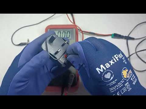
Channel: How2 (476 subscribers)
This is the strongest pick in a fairly weak batch — most of the other candidates are either shorts, PC build clickbait, or vague sponsored content. A proper teardown and bench test of a budget 12V wall-wart adapter is genuinely educational territory, and small-channel reviewers in this niche (think a smaller-scale BigClive or DiodeGoneWild) tend to do the kind of hands-on engineering critique that's hard to find elsewhere.
What makes this format worth watching is that cheap plug-in supplies are everywhere in hobbyist and IoT projects, but their actual specs are rarely what the label claims. A good review covers the real output voltage under load, ripple on the scope, transformer vs. switch-mode topology, the quality of the smoothing capacitors, isolation between mains and low-voltage side, and whether the build meets the safety claims printed on the case. These are exactly the things you need to evaluate before trusting a $5 adapter to power something you care about.
For anyone building circuits, the takeaways translate directly: how to spot a sketchy supply, what ripple is acceptable for digital vs. analog loads, and why "12V 1A" on a label doesn't always mean 12V at 1A. The channel is tiny (476 subs), which is exactly the kind of independent voice this curation aims to surface.
Daily YT Engineering
Lec03: Thermodynamic Analysis of Vapor Power Cycle #swayamprabha
2026-06-12

Channel: CH 27: IIT KANPUR 04: Mechanical Engineering... (682 subscribers)
Most of today's candidates are 10-to-30-second Shorts that toss out a single sentence and call it a lesson. This IIT Kanpur lecture is the opposite — it's a full classroom session from the institute's Power Plant System Engineering course, broadcast via India's Swayam Prabha educational initiative.
The topic, thermodynamic analysis of the vapor power cycle, is the foundational engineering behind essentially every thermal power station on Earth: coal, nuclear, concentrated solar, and combined-cycle gas plants all run some variant of the Rankine cycle. Expect a treatment of the four-stage cycle (boiler, turbine, condenser, feed pump), T-s and h-s diagrams, work and heat calculations across each stage, and the efficiency penalties imposed by real-world irreversibilities. Earlier lectures in the series likely set up the ideal Carnot benchmark, so this one should bridge from textbook idealization to the practical Rankine modifications engineers actually deploy.
It's not flashy — it's a chalkboard-and-equations academic lecture from a tier-one engineering institute, delivered to a tiny audience. But if you want to actually understand why a steam plant looks the way it does, instead of just being told "entropy goes up" in ten seconds, this is the real thing.
Daily YT Maker
DIY French Cleat Belt Sander Holder | Free CNC Files & Workshop Organization
2026-06-12

Channel: Nine Finger Woodworking (841 subscribers)
Workshop organization is one of those projects that pays dividends every single time you walk into the shop, and a French cleat system is the gold standard for flexible, reconfigurable tool storage. This build tackles a specific pain point that nearly every woodworker faces: where do you actually put a belt sander? It's heavy, awkwardly shaped, has a dangling cord, and tends to live in whatever drawer or shelf it last got shoved into.
What makes this video worth watching over the dozens of generic French cleat tutorials is the combination of a real, specific tool problem with free downloadable CNC files. You get to see both the design thinking — how the holder cradles the sander, manages the cord, and locks onto the cleat — and the fabrication workflow on a CNC. That's a useful pairing: even if you don't have a CNC, watching how the file is structured teaches you something about translating a 3D shop problem into a 2D toolpath.
Nine Finger Woodworking is a small channel (under 1k subs) genuinely sharing project files rather than gating them behind a Patreon, which is increasingly rare. The full-length version (not the short companion clip) should give enough process detail to actually replicate the build or adapt the approach for other awkward tools — palm routers, drills, heat guns — sitting homeless in your shop.
Daily YT Welding
Which Welding Type Do You Actually Need? tips quick choose types of welding and their applications
2026-06-12

Channel: kanopirumahku steel fabrication (558 subscribers)
Honest disclaimer: this batch is unusually thin — most candidates are hashtag-spam Shorts from channels recycling the same SEO description block. This video from kanopirumahku steel fabrication is the least bad of the bunch because it at least promises a structured comparison rather than 15 seconds of bead footage.
The premise is the question every beginner asks before buying their first machine: MIG, TIG, or Stick — which one do I actually need? A good answer covers more than marketing bullet points. MIG (GMAW) wins on speed and ease of learning, making it the default for auto-body and general fab on clean steel. TIG (GTAW) gives precise, clean welds on thin material and non-ferrous metals like aluminum and stainless, but the learning curve is steep and travel speed is slow. Stick (SMMA) is the workhorse for dirty, rusty, or outdoor work where wind would blow shielding gas away.
If the video walks through these tradeoffs — amperage ranges, material thickness sweet spots, shielding gas vs. flux, and indoor vs. outdoor suitability — it's a useful 5-minute primer before committing to a machine that costs hundreds or thousands of dollars. Watch with skepticism and cross-reference any specific amperage claims against your filler metal's spec sheet.
